The normal distribution
The normal distribution · Diagrams · Complete reading
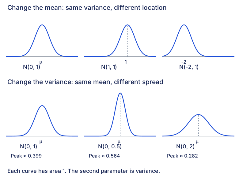
Location and spread
Expand diagramFit diagram to page
Use the scrollbars or arrow keys to inspect details.
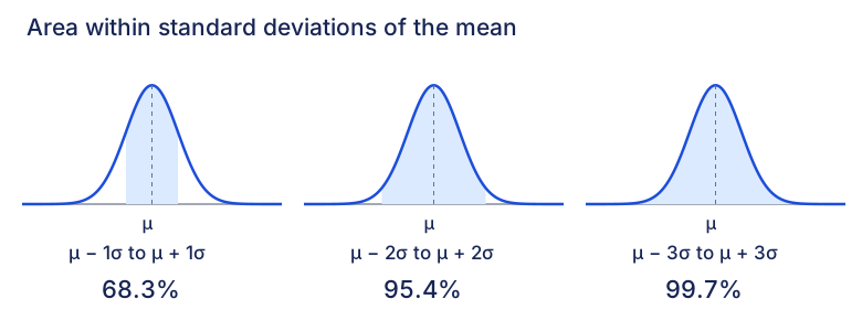
Areas within standard deviations
Expand diagramFit diagram to page
Use the scrollbars or arrow keys to inspect details.
Method map: Translate a normal event before calculating
Identify the model and its spread, keep the event when standardising, then match the calculation to the shaded area. An interval probability and a density height are different quantities.
Read the spread before entering a calculator value
In the variance convention N(μ, σ²), the second parameter is the variance. Standardisation requires a positive standard deviation.
Expand diagramFit diagram to page
Use the scrollbars or arrow keys to inspect details. The text explanation follows.
- Variance v is givenUse σ = √v
For a model , enter standard deviation 5. Do not enter 25 as the standard deviation.
- Standard deviation is givenUse it directly
For , the standard deviation is 6 and the variance is 36. Label the parameter rather than guessing from the size of the number.
Check that the normal model is stated or justified in context. A zero spread does not give a nondegenerate standard normal variable and cannot be used as the divisor here.
Transform every cutoff and preserve the event
Define Z from the same variable X. Subtract the mean and divide every bound by the positive standard deviation; the inequality directions stay unchanged.
- Left or right tailKeep the shaded side
The event becomes ; the event becomes . A right-tail event does not turn into a left-tail event merely because the variable is standardised.
- Between two boundsTransform both endpoints
For , set and . The event is , with the same probability. With a nondegenerate normal model, including an individual endpoint does not change that probability.
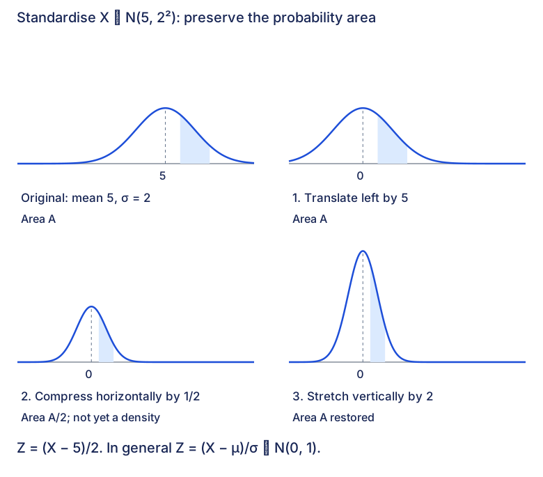
The source density stages have areas , , , then . Horizontal compression of a drawn density alone changes its area; the compensating vertical stretch restores a normalised density. Compare the four stages and their labelled areas in the source figure.
Choose an area calculation or an inverse cutoff
Decide whether the unknown is a probability or a cutoff. Sketch the shaded region and name the calculator's area convention before using it.
- Known cutoffsCalculate the probability of the event
For a standardised cutoff z, a left area is and a right area is . For the standardised interval , use . For a direct normalcdf calculation, use the original bounds with μ and σ, or the standardised bounds with mean 0 and standard deviation 1. Do not mix those two parameter sets.
- Known one-sided probability pMatch the inverse to the tail
For , a lower-tail-only inverse uses p for a stated left area and 1−p for a stated right area. When a standard-normal inverse returns z, recover the original cutoff with . An inverse supplied with the original μ and σ already returns the original cutoff. An interface with an explicit RIGHT selector may instead use the right area directly; do not complement it twice.
- Known central probability pUse symmetry only when justified
For a central interval symmetric about the mean and , the lower-tail endpoint areas are and . CENTER returns endpoints, not the half-width. An arbitrary interval is not determined by its area alone.
Check whether a cutoff should be above or below the mean and substitute back into the original event. Keep full calculator precision until the final requested rounding. A density height is not a probability.
Try a worked example
Read a case, make a prediction, then reveal the reasoning. The examples keep their stated values.
A large right area gives a cutoff below the mean
The source gives and . Before calculating, predict which side of 100 contains b.
Show reasoning
1. Identify the spread and shade the stated area
The standard deviation is 6, not the variance 36. More than half the curve lies to the right of b, so b is below the mean.
2. Complement only for a lower-tail interface
A RIGHT-tail interface can use the given 0.770 directly. A lower-tail-only inverse uses the complementary area 0.230. Both describe the same cutoff.
3. Recover the cutoff and check its direction
Keep calculator precision until the source’s final rounding to three significant figures. The result is below 100 as predicted.
A central interval has two endpoints and one half-width
The source gives and . Find the central interval, then distinguish its endpoints from the half-width a.
Show reasoning
1. Expand the event and split the remaining area
The standard deviation is the positive square root of 25, namely 5. The interval has probability 0.8 and its bounds are symmetric about 70, so the remaining 0.2 splits into tails of 0.1.
2. Use lower-tail areas 0.1 and 0.9
A CENTER interface returns the pair of endpoints; the two lower-tail inverse calculations return the same pair. Neither returned endpoint is a itself.
3. Find the half-width separately
Either endpoint gives the same half-width. The source reports a = 6.41 and interval limits 63.6 and 76.4, all to three significant figures. Retain the full endpoint values until rounding.
Compare with the density transformation
Expand diagramFit diagram to page
Use the scrollbars or arrow keys to inspect details.
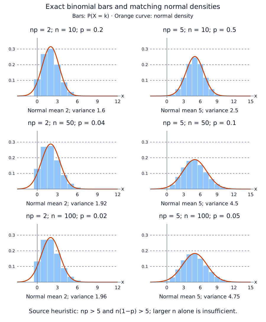
Six source binomial-to-normal comparisons
Expand diagramFit diagram to page
Use the scrollbars or arrow keys to inspect details.