Sequences and series

Read terms, positions and partial sums

A sequence is an ordered list. The source gives the finite lists $3,4,5,6,7$ and $1,1/2,1/3,1/4,1/5$, and the infinite lists $2,4,6,8,\ldots$ and $1,1,2,3,5,8,13,21,\ldots$. In the first list, the first term is 3, the second 4 and the fifth and last 7. An ellipsis indicates continuing terms; a finite sequence has a last term. The source links Fibonacci music through its QR code.

In $u_1,u_2,u_3,\ldots,u_n,\ldots$, the subscript is the index, meaning position. Here $n$ is a positive integer, as the Teacher emphasises. Adding terms gives a series; its partial sum is

$$S_n=u_1+u_2+\cdots+u_n.$$

An explicit formula $u_n=f(n)$ takes the position as input and produces that term. A finite sequence has a finite domain such as $\{1,2,3,4,5\}$; an infinite sequence can have domain $\mathbb Z^+$. This qualifies the source’s Function callout: a finite list does not have a term at every positive index. For $u_n=n^2+3$, substituting $n=1,2,3,4,5$ gives $4,7,12,19,28$, and $u_{100}=100^2+3=10003$. Self-Practice 1 checks both substitution and choosing a formula with the correct domain.

The supplied calculator instructions use the device shown in the source:

1. Press MODE and choose SEQ.
2. Press y=, enter $u(n)=n^2+3$ using the X,T,θ,n key for $n$, and set nMin=1. The explicit formula does not need the $u(1),u(2)$ initial-value fields filled.
3. Press 2nd graph to view the table, using Up/Down to inspect indices. The displayed index 0 gives ERROR because of the stated sequence domain; the polynomial itself is mathematically evaluable at 0, but that would extend this sequence’s domain.
4. Press 2nd window and set TblStart=100 rather than scrolling from the beginning.
5. Press 2nd graph again. The source’s table 100–110 gives $10003,10204,10407,10612,10819,11028,11239,11452,11667,11884,12103$.

Its first table shows indices 1–10 with $4,7,12,19,28,39,52,67,84,103$. These finite tables illustrate increase. Algebra proves it for all positive indices: $u_{n+1}-u_n=2n+1>0$; the values also grow without bound. A calculator table is evidence for a conjecture, not a proof about infinitely many terms.

The source outline sets out the later chapter route: finite/infinite sequences and series; sequences as positive-integer-input functions; the relation between $u_n$ and $S_n$; explicit formulas; recurrences $u_{n+1}=f(u_n)$; sigma notation; sums/differences of series; convergence and infinite sums; arithmetic nth-term/finite-sum formulas; geometric nth-term/finite-sum formulas; geometric convergence conditions; and the convergent geometric infinite-sum formula. The opening material here does not replace those later source sections.

Separate behaviour from convergence

Ask two independent questions: does each term rise or fall, and do the terms approach one finite value? In the source’s strict terminology, increasing means $u_{n+1}>u_n$ and decreasing means $u_{n+1}<u_n$. A sequence may be neither.

Write

$$\lim_{n\to\infty}u_n=L$$

when the terms approach one finite constant $L$. Read lim as “the limiting value of”, the arrow as “approaches” or “tends to”, $u_n$ as the sequence formula, and $L$ as the limiting value.

The complete statement reads “the limit of the sequence $u_n$ as $n$ tends to infinity is $L$”. This notation reappears in differentiation.

A sequence is convergent when such a finite limit exists and divergent otherwise; $u_n\to+\infty$ describes divergence, not a finite limit.

The source’s Limits callout also discusses a series’ limiting sum. Keep the objects separate: sequence convergence concerns $u_n$, while convergence of a series concerns the sequence of partial sums $S_n$. A sequence’s terms tending to zero alone does not establish that their series has a finite sum.

Both printed lists for $-n^2$ skip $-16$; it is restored above from the formula. The printed “$w_n\to-1$ or $1$” describes the two alternating values, not one sequence limit. Its odd and even subsequences have different limits, so the whole sequence diverges.

Example 1 shows why the two questions must stay separate. The alternation $(-1/2)^n$ converges to 0 because its magnitude tends to 0, while $(-2)^n$ diverges because its magnitudes grow without bound.

The sequence $2+e^{-n}$ decreases to 2. Its exact terms are greater than 2 for every finite positive index, even when the calculator displays 2 after rounding.

The Teacher asks you to notice this limitation.

Likewise, the displayed starting index 100 is an arbitrary sample, not a mathematical infinity or cutoff.

Apply limit laws with their hypotheses

If $u_n\to A$ and $v_n\to B$ with finite $A,B$, the source laws are

$$\lim_{n\to\infty}(u_n\pm v_n)=A\pm B,\qquad \lim_{n\to\infty}(c u_n)=cA$$

for a constant $c$, and

$$\lim_{n\to\infty}\frac{u_n}{v_n}=\frac AB\quad\text{provided }B\ne0.$$

Check these hypotheses before substituting limits. The source warns against treating $0/\infty$, $\infty/\infty$ or $0/0$ as ordinary real-number divisions. Infinity is not a real number. In limit analysis, a numerator tending to 0 over a denominator whose magnitude tends to infinity does tend to 0; the warning does not forbid that conclusion. The forms $0/0$ and $\infty/\infty$ alone are inconclusive and require rewriting the sequence.

Rewrite rational formulas before taking limits

Example 2 deliberately forbids a calculator. Divide numerator and denominator by a suitable power of $n$, or use long division to expose a polynomial plus a proper rational remainder. For positive $n$, $3n-1$ is nonzero.

In(a), expanding the squared denominator and dividing by $n^2$ gives

$$\frac{2n+1}{(3n-1)^2} =\frac{2/n+1/n^2}{9-6/n+1/n^2}\to0.$$

In(b), both printed methods give the same finite limit:

$$\frac{2n+1}{3n-1}=\frac23+\frac5{3(3n-1)} =\frac{2+1/n}{3-1/n}\to\frac23.$$

In(c), long division gives

$$\frac{6n^2+n+1}{3n-1}=2n+1+\frac2{3n-1}.$$

The proper rational remainder tends to 0, but $2n+1$ grows without bound, so the whole sequence diverges to $+\infty$. The full solutions retain every printed intermediate step and both methods for (b).

Generate a sequence from earlier terms

A recurrence relation expresses a term using one or more previous terms, together with enough initial values to start. The source shows $u_{n+1}=f(u_n)$ as a common form. Recurrences can also depend explicitly on $n$ or on two preceding terms, as its examples demonstrate. An explicit formula takes the index as input directly; a recurrence advances through earlier terms.

The three source examples pair a recurrence with an explicit formula:

• Squares: $u_{n+1}=u_n+2n+1$, $u_1=1$, gives $1,4,9,16,25,36,\ldots$ and $u_n=n^2$. Indeed, $(n+1)^2-n^2=2n+1$.
• Harmonic sequence: $1/u_{n+1}=1/u_n+1$, $u_1=1$, gives $1,1/2,1/3,1/4,1/5,\ldots$ and $u_n=1/n$. The reciprocals increase by one. Its terms are nonzero; this name describes the sequence, not a claim that its infinite series has a finite sum.
• Fibonacci sequence: $u_n=u_{n-1}+u_{n-2}$ for $n\ge3$, with $u_1=u_2=1$, gives $1,1,2,3,5,8,13,21,34,\ldots$. Two initial terms are needed here. Its printed explicit formula is

$$u_n=\frac1{\sqrt5}\left[\left(\frac{1+\sqrt5}{2}\right)^n-\left(\frac{1-\sqrt5}{2}\right)^n\right].$$

The source gives this formula without deriving it. The recurrence supplies a simple way to generate its integer terms without approximating the square roots.

Match the calculator setup to the recurrence

Example 3 uses $u_n=2u_{n-1}+3$, $u_1=2$. Start at the given first term and apply the relation from $n=2$ onwards. On the device shown in the source:

1. Press MODE and choose SEQ.
2. Press y=, select the current-term form SEQ(n) and set nMin=1.
3. Press 2nd 7 for the $u$ function and enter $2u(n-1)+3$; use X,T,θ,n for $n$.
4. Set u(1)=2. The source leaves u(2) blank because the recurrence computes it from the given first term.
5. Press 2nd graph and inspect the table with Up/Down. Its first eleven terms are $2,7,17,37,77,157,317,637,1277,2557,5117$.

The requested $u_{20}=2621437$ comes after nineteen updates. The worked solution also gives an independent shifted-form check; that algebra supplements the printed calculator method.

Example 4 starts with $u_{n+1}-3u_n=4$, $u_1=5$. Isolate the next term first:

$$u_{n+1}=3u_n+4.$$

For the source’s second method, keep the calculator in SEQ mode, press y=, use Up/Right to highlight TYPE SEQ(n+1) and press Enter. Set nMin=1; use 2nd 7 for $u$, X,T,θ,n for $n$, enter $3u(n)+4$, and set u(1)=5. 2nd graph with Up/Down gives $5,19,61,187,565,1699,5101,15307,45925,137779,413341$ at indices 1–11. Its requested first three new terms agree with direct substitution. The recurrence notation and the selected calculator type must describe the same update.

Recognise arithmetic progressions

An arithmetic progression (AP) has a constant difference between consecutive terms:

$$u_{n+1}-u_n=d.$$

The common difference $d$ may be positive, negative or zero. With first term $a$, each next term is obtained by adding $d$. The source’s Models callout connects this to quantities that repeatedly change by a fixed added amount.

The unnumbered source activity has three lists: $2,7,12,17,22$ with $a=2,d=5$; $13,10,7,4,1$ with $a=13,d=-3$; and $-14,-11,-8,-5,-2$ with $a=-14,d=3$. Its follow-up question $2,-4,6,-8,10$ is not an AP: the first two consecutive differences are $-6$ and $10$. A regular-looking sign pattern is not enough to establish an AP.

The source builds the general term by matching positions to additions:

There are $n-1$ additions after the first term, so

$$u_n=a+(n-1)d,\qquad n\in\mathbb Z^+.$$

A negative difference gives a decreasing AP; a zero difference gives a constant AP. The sign of the first term does not determine the sign of the difference.

Use the arithmetic nth-term formula

Example 5 retains both complete first-term/difference/formula rows. For $-3,-8,-13,\ldots$, $a=-3,d=-5$ and $u_n=2-5n$. For $1,2\frac12,4,5\frac12,7,\ldots$, $a=1,d=3/2$ and $u_n=(3/2)n-1/2$. Self-Practice 2 then substitutes specified indices using $a=2,d=0.5$.

The next examples ask three different questions:

• Find a term (Example 6): identify $a=7,d=6$ and evaluate $u_{20}=7+19(6)=121$.
• Count terms (Example 7): treat the final value 3 as $u_n$ and solve $57+(n-1)(-3)=3$. The result is $n=19$ terms, including both endpoints. Eighteen is the number of gaps.
• Recover the progression (Example 8): translate the third and tenth terms into $a+2d=10$ and $a+9d=24$. Subtraction gives $7d=14$, hence $d=2$ and $a=6$.

In a counting problem, the resulting index must be a positive integer and really produce the stated final term. For sums of many terms, use the AP and GP sum formulas in the later methods.

Prove a progression and relate three terms

An AP test must work for every neighbouring pair in the stated domain:

$$u_{n+1}-u_n=d,$$

where the difference is independent of $n$. Equivalently, $u_n-u_{n-1}=d$ where both terms exist. This is also a recurrence relation. Checking the first two differences alone does not prove the claim for an infinite sequence.

The source challenges an argument for $u_n=2+3n$: its first terms are $5,8,11$, and their two consecutive differences are $3$. The conclusion that this is an AP is true, but that finite check is not a valid proof. Use the general neighbouring terms instead:

$$u_{n+1}-u_n=(2+3(n+1))-(2+3n)=3.$$

The general calculation completes the printed explanation. For three consecutive AP terms $x,y,z$, equating the two differences gives

$$y-x=z-y=d\quad\Longrightarrow\quad y=\frac{x+z}{2}.$$

The middle term is the arithmetic mean of its neighbours. This relation is useful when an AP problem gives information about three successive terms.

Recognise and generate geometric progressions

A geometric progression (GP) in this lecture consists of nonzero terms with a nonzero constant consecutive ratio:

$$\frac{u_{n+1}}{u_n}=r.$$

The common ratio can be positive or negative. With first term $a$, multiply by $r$ to obtain each next term. The Teacher’s Models callout connects this to a quantity changing repeatedly by a fixed percentage or ratio, whereas an AP models a fixed added amount.

The source table gives $5,25,125,625$ with $a=5,r=5$; $27,9,3,1,1/3,1/9,1/27$ with $a=27,r=1/3$; and $2,-6,18,-54,162$ with $a=2,r=-3$. The following question $2,4,6,10,14$ is not a GP: $4/2=2$ but $6/4\ne2$.

There are $n-1$ multiplications after the first term, so

$$u_n=ar^{n-1},\qquad n\in\mathbb Z^+.$$

Example 9 retains both complete table rows: $-1,2,-4,8,-16,\ldots$ has $a=-1,r=-2$ and $u_n=(-1)(-2)^{n-1}=\tfrac12(-2)^n$; $1,1/2,1/4,1/8,1/16,\ldots$ has $a=1,r=1/2$ and $u_n=1(1/2)^{n-1}=(1/2)^{n-1}$. Self-Practice 3 uses $a=10,r=2/3$ to find $u_6\approx1.32$ and $u_{13}\approx0.0771$. Keep the ratio exact until rounding the results.

Solve geometric term and threshold problems

Example 10 uses $a=2,r=8$, so $u_n=2(8)^{n-1}$ and $u_7=524288$. To find the first term exceeding one million, retain an exact inequality until the final integer choice:

$$\begin{aligned} 2(8)^{n-1}&>1000000,\\ 8^{n-1}&>500000,\\ (n-1)\ln8&>\ln500000,\\ n&>1+\frac{\ln500000}{\ln8}\approx7.31. \end{aligned}$$

The least integer is $8$. The source also displays $n-1>6.31$ and $n>7.31$ as rounded cutoffs; these do not replace the exact logarithmic inequality.

For its calculator method, enter Y1=2*8^(X−1) and inspect the table. The source explicitly requires showing the supporting values:

Highlight the Y1 value to read its actual integer. The Teacher warns against copying the rounded screen value 4.19E6 instead of 4194304. Since the terms increase, checking the two adjacent terms 7 and 8 establishes the first crossing. The screenshot’s X=0 row is a calculator sample; this sequence’s domain still starts at n=1.

Example 11 reverses the task: from $u_3=36$ and $u_6=243/2$, write

$$ar^2=36\quad\text{(1)},\qquad ar^5=\frac{243}{2}\quad\text{(2)}.$$

The illustrated source callout explains why division is useful: (2) divided by (1) eliminates the unknown first term $a$. It gives $r^3=27/8$, hence $r=3/2$. Substitute into either equation to recover $a$; using (1), $a=36/(3/2)^2=16$. The divisor is nonzero because the given third term is 36.

Compare AP and GP tests and constant sequences

A GP proof must show that $u_{n+1}/u_n$ is independent of $n$ for every valid neighbouring pair, with nonzero terms. Equivalently use $u_n/u_{n-1}=r$ where defined. The source asks why $u_2/u_1=u_3/u_2$ alone is insufficient: as in the AP argument, it tests only two pairs.

For three consecutive GP terms $x,y,z$,

$$\frac yx=\frac zy=r\quad\Longrightarrow\quad y^2=xz.$$

When all three terms are nonnegative, $y=\sqrt{xz}$ is the geometric mean of $x$ and $z$. Keep that sign condition: $y^2=xz$ alone does not choose the positive square root. The lecture’s nonzero GP convention also excludes zero denominators.

A constant sequence has all its terms equal. The source examples are $1,1,1,1,1,1,1,\ldots$ and the finite list $0,0,0,0,0,0,0$. Its unnumbered question about $2,2,2,\ldots,2$ has both classifications: AP with $a=2,d=0$, and GP with $a=2,r=1$. A zero constant sequence is an AP with difference zero, but it is excluded from GP under this lecture’s nonzero-term definition.

Recover a sequence from its partial sums

A series adds the terms of a sequence. A finite series stops after finitely many terms, such as $2+4+6+8+10$. An infinite series continues indefinitely, such as $1+2+4+8+16+\cdots$; calling it infinite does not assert a finite sum.

Let $S_n$ be the sum of the first $n$ terms. The source derives the connection by subtraction:

$$\begin{aligned} S_n&=u_1+u_2+\cdots+u_{n-1}+u_n&&\text{(1)},\\ S_{n-1}&=u_1+u_2+\cdots+u_{n-1}&&\text{(2)},\\ S_n-S_{n-1}&=(u_1+u_2+\cdots+u_{n-1}+u_n)\\ &\quad-(u_1+u_2+\cdots+u_{n-1})\\ &=u_n. \end{aligned}$$

The shared first $n-1$ terms cancel. Therefore

$$u_n=S_n-S_{n-1}\quad(n\ge2),\qquad u_1=S_1.$$

Treat the first term separately rather than assuming an unspecified $S_0$. The related cumulative-sum question below applies this method with a particular formula. These term-to-sum relationships also help when applying summation laws and AP/GP sum formulas.

Check the first term after subtracting partial sums

Example 12 applies $u_n=S_n-S_{n-1}$ for $n\ge2$, then checks $u_1=S_1$ separately. With $S_n=2^n-1$, subtraction gives $u_n=2^{n-1}$; at n=1 this gives 1, which agrees with S1. The general ratio $u_{n+1}/u_n=2$ proves the terms form a GP.

For $S_n=n^2+3n$, the result is $u_n=2n+2$ for n≥2. Its n=1 value 4 agrees with S1, so the formula holds for every positive index. The general difference is $[2(n+1)+2]-(2n+2)=2$, proving an AP. The illustrated source callout asks you to show the common difference or ratio for general neighbouring terms, rather than simply presenting a familiar AP/GP-looking formula.

The extra constant in $S_n=n^2+3n+1$ cancels in the subtraction, but it changes the first term:

$$u_n=\begin{cases}5&n=1,\\2n+2&n\ge2.\end{cases}$$

The first three terms are 5,6,8. Their consecutive differences 1 and 2 disagree, as do their ratios 6/5 and 8/6. The full sequence is neither AP nor GP, even though its tail from the second term is arithmetic. The full worked exercise retains each printed expansion and first-term check.

Read every part of sigma notation

The Greek capital letter $\Sigma$, pronounced sigma, represents a sum. The source introduces it through $3^2+4^2+5^2+6^2+7^2+8^2+9^2$. Three pieces of information specify this sum: its general term, lower bound and upper bound. The source’s labelled notation diagram has four labels:

This table gives a text equivalent of all the diagram’s labels. For integer bounds $m\le n$,

$$\sum_{r=m}^{n}u_r=u_m+u_{m+1}+\cdots+u_{n-1}+u_n.$$

In the opening example,

$$\sum_{r=3}^{r=9}r^2=\sum_{r=3}^{9}r^2=3^2+4^2+5^2+6^2+7^2+8^2+9^2.$$

Read this as “the sum of all terms of the form r squared, where r takes each integer value from 3 to 9 inclusive”. Omitting the repeated r= above sigma does not change the meaning. The index need not be r: $\sum_{k=1}^{5}k^2=\sum_{r=1}^{5}r^2$, and

$$\sum_{r=1}^{n}(2r+1)=\sum_{k=1}^{n}(2k+1)=\sum_{i=1}^{n}(2i+1).$$

Only the bound counter and its matching occurrences are renamed. The source’s Equivalence callout notes that different sigma forms can make simplification and manipulation easier.

Change the counter together with the bounds

Sigma expressions are not unique. The source gives

$$\sum_{r=1}^{10}r=\sum_{r=0}^{9}(r+1)$$

and, for a positive integer n,

$$\sum_{r=1}^{2n}r(r+1) =\sum_{r=0}^{2n-1}(r+1)(r+2) =\sum_{r=-2n-1}^{-2}r(r+1).$$

The source ends these equalities with ellipses, not a supplied evaluated answer. The last form runs through the same products in reverse order: set $r=-k-1$ to obtain $r(r+1)=k(k+1)$. This substitution is an authored explanation of the printed equivalence. Integer counters can be zero or negative when the formula is defined; their bounds need not start at one.

Typical term patterns are $2r$ for even integers, $2r+1$ or $2r-1$ for odd integers, and $(-1)^r$, $(-1)^{r+1}$ or $(-1)^{r-1}$ for alternating signs. Choose the exponent to match the first sign at the chosen starting index. Check both endpoint substitutions whenever you change the formula or limits.

Expand, count and construct sums

With finite integer bounds, including both endpoints gives

$$\text{number of terms}=n-m+1\qquad\text{in }\sum_{r=m}^{n}u_r.$$

Example 13 expands six integers from 1 to 6, four squares from 5 to 8, five terms of $2k-1$ from 0 to 4, and infinitely many powers $(1/2)^r$ from 0 onwards. The last expansion starts with $(1/2)^0=1$. Its infinite number of terms does not by itself tell you the sum’s value.

Example 14 constructs the formula and its bounds together. The AP $1+4+7+10+\cdots+88$ has $a=1,d=3$, so $u_n=1+(n-1)3=3n-2$. Solving $88=1+(n-1)3$ gives 30 terms and $\sum_{r=1}^{30}(3r-2)$.

For the odd terms through 99, the two printed methods give

$$\sum_{r=1}^{50}(2r-1)=\sum_{r=0}^{49}(2r+1).$$

The position-one nth-term formula is $u_n=2n-1$; a counter starting at 0 instead uses $v_j=2j+1$, $0\le j\le49$. The source calls both formulas u_n; the different letters here make the change of indexing explicit rather than giving two values to one position.

For $-2+3-4+5-\cdots+41$, the two printed methods give

$$\sum_{r=1}^{40}(-1)^r(r+1)=\sum_{r=2}^{41}(-1)^{r+1}r.$$

The first indexing has $u_n=(-1)^n(n+1)$, $1\le n\le40$; the shifted magnitude counter has $v_j=(-1)^{j+1}j$, $2\le j\le41$. Both begin at −2 and finish at +41. The illustrated source guidance stresses checking an expression by substituting its indices for each term.

Self-Practice 4 retains both printed alternatives for each series:

$$1^4+2^4+\cdots+n^4+(n+1)^4 =\sum_{r=1}^{n+1}r^4=\sum_{r=0}^{n}(r+1)^4,$$ $$-1+2-3+4-5+6 =\sum_{r=1}^{6}(-1)^r r =\sum_{r=2}^{7}(-1)^{r-1}(r-1).$$

The working panels keep all original methods and term-count results. Do not replace a requested expansion with only its numerical total.

Evaluate a finite sum with the supplied calculator

The source illustrates $\sum_{r=2}^{8}r^4(r-1)$ using its calculator:

1. Press MATH, scroll to option 0 (summation). Alternatively press ALPHA WINDOW, then choose option 2.
2. Enter lower limit 2, upper limit 8 and formula X^4(X−1). X is the calculator’s counter corresponding to the written r.
3. Press Enter. The displayed result is 53004.

The original menu, template/input and result screens are retained in the illustration archive. The worked exercise also gives an independent seven-term arithmetic check.

Self-Practice 5 prints three results: the fifteen squares $1^2+2^2+\cdots+15^2$ sum to 1240; $\sum_{r=1}^{20}(3-2r)=-360$; and $\sum_{r=0}^{15}2^r=65535$. The last has sixteen terms because it includes index 0. Its working shows cancellation after doubling. Summation laws and AP/GP sum formulas provide further ways to evaluate larger sums.

Find a least index from partial sums

Example 15 asks for the least positive integer $n$ with $H_n=\sum_{r=1}^{n}1/r>4$. The source enters a summation in Y1, using X for its upper bound and a separate R as the counter:

$$Y_1(X)=\sum_{R=1}^{X}\frac1R.$$

Its displayed table has these values, retaining the screen’s precision:

The illustrated guidance requires a supporting table when using this calculator method. The printed written table gives $H_{30}\approx3.995<4$, $H_{31}\approx4.027>4$ and $H_{32}\approx4.059>4$. The last rounded value is a source error: the unrounded $H_{32}\approx4.058495195437$ rounds to 4.058 at three decimal places. Avoid rounding an already rounded display a second time.

Each additional reciprocal is positive, so the partial sums strictly increase. Since $H_{30}<4<H_{31}$, the least index is 31. This monotonicity argument explains why checking the neighbouring values establishes the first crossing; it supplements the printed calculator evidence.

Apply and prove summation laws

For finite integer bounds $m\le n$ and constant $c$, a constant factor can be taken outside a sum:

$$\begin{aligned} \sum_{r=m}^{n}cu_r &=cu_m+cu_{m+1}+\cdots+cu_n\\ &=c(u_m+u_{m+1}+\cdots+u_{n-1}+u_n)\\ &=c\sum_{r=m}^{n}u_r. \end{aligned}$$

The source’s examples keep their original bounds:

$$\sum_{r=1}^{10}2r=2\sum_{r=1}^{10}r,\qquad \sum_{r=12}^{100}3r^2=3\sum_{r=12}^{100}r^2.$$

Sums and differences can also be separated over the same bounds. The source proves addition by expanding and regrouping:

$$\begin{aligned} \sum_{r=m}^{n}(u_r+v_r) &=(u_m+v_m)+(u_{m+1}+v_{m+1})+\cdots\\ &\quad+(u_{n-1}+v_{n-1})+(u_n+v_n)\\ &=(u_m+u_{m+1}+\cdots+u_{n-1}+u_n)\\ &\quad+(v_m+v_{m+1}+\cdots+v_{n-1}+v_n)\\ &=\sum_{r=m}^{n}u_r+\sum_{r=m}^{n}v_r. \end{aligned}$$

For subtraction, regroup the negative terms with their signs intact:

$$\begin{aligned} \sum_{r=m}^{n}(u_r-v_r) &=(u_m-v_m)+(u_{m+1}-v_{m+1})+\cdots\\ &\quad+(u_{n-1}-v_{n-1})+(u_n-v_n)\\ &=(u_m+u_{m+1}+\cdots+u_{n-1}+u_n)\\ &\quad-(v_m+v_{m+1}+\cdots+v_{n-1}+v_n)\\ &=\sum_{r=m}^{n}u_r-\sum_{r=m}^{n}v_r. \end{aligned}$$

The two printed examples are

$$\sum_{r=1}^{3}(r+e^r)=\sum_{r=1}^{3}r+\sum_{r=1}^{3}e^r,$$ $$\sum_{r=12}^{88}(r-r^2)=\sum_{r=12}^{88}r-\sum_{r=12}^{88}r^2.$$

These rules do not say that a sum of products equals the product of two sums.

Remove a prefix and restore missing terms

To isolate a tail when $k<m\le n$, subtract the excluded prefix:

$$\sum_{r=m}^{n}u_r=\sum_{r=k}^{n}u_r-\sum_{r=k}^{m-1}u_r.$$

The source proves this by adding and subtracting the same prefix. Write its two groups as

$$\begin{aligned} A&=u_k+u_{k+1}+\cdots+u_{m-2}+u_{m-1},\\ B&=u_m+u_{m+1}+\cdots+u_{n-1}+u_n. \end{aligned}$$

Then its cancellation argument is

$$\begin{aligned} \sum_{r=m}^{n}u_r&=B=A+B-A\\ &=(u_k+u_{k+1}+\cdots+u_{m-2}+u_{m-1}\\ &\quad+u_m+u_{m+1}+\cdots+u_{n-1}+u_n)-A\\ &=\sum_{r=k}^{n}u_r-\sum_{r=k}^{m-1}u_r. \end{aligned}$$

The letters A and B organise the same printed expansion into shorter lines. As with any ellipsis, include each actual term once when the ranges are short. The source notes that this is useful when a formula for the prefix from 1 is given but the required sum starts at $k+1$: subtract the first k terms.

Both printed rule examples retain their exact excluded prefixes:

$$\sum_{r=4}^{10}r=\sum_{r=1}^{10}r-\sum_{r=1}^{3}r,$$ $$\sum_{r=10}^{100}\frac1{r(r-1)} =\sum_{r=2}^{100}\frac1{r(r-1)}-\sum_{r=2}^{9}\frac1{r(r-1)}.$$

Example 16 asks you to supply missing terms: remove $1^2$ to move a square sum’s lower bound from 1 to 2; remove $\sum_{r=2}^{4}1/(r+1)$ to move a reciprocal sum from 2 to 5; add $\sum_{n=1}^{2}2/n$ to restore the first two terms of a sum starting at 3. Adding or subtracting terms is another way to obtain equivalent sigma expressions, alongside changing the counter.

Match a shifted sum to a given identity

Example 17 gives

$$\sum_{n=1}^{N}\frac1{n(n+1)(n+2)} =\frac14-\frac1{2(N+1)}+\frac1{2(N+2)}$$

and asks for $\sum_{n=3}^{N}1/[n(n-1)(n-2)]$, with integer $N\ge3$. Its two methods make the same change visible in different ways.

List the terms: the first terms have denominators $3\cdot2\cdot1$, $4\cdot3\cdot2$, $5\cdot4\cdot3$. Reorder each product to match $1\cdot2\cdot3$, $2\cdot3\cdot4$, $3\cdot4\cdot5$, and continue through $(N-2)(N-1)N$. There are $N-2$ terms, so apply the supplied identity with upper bound N−2, not N.

Change the counter: let $r=n-2$, giving $n-1=r+1$ and $n=r+2$. The illustrated source guidance uses a new letter to prevent confusion and aims to match the given formula with lower index 1. Transform both endpoints: $n=3$ gives $r=1$, while $n=N$ gives $r=N-2$. Thus

$$\begin{aligned} \sum_{n=3}^{N}\frac1{n(n-1)(n-2)} &=\sum_{r=1}^{N-2}\frac1{(r+2)(r+1)r}\\ &=\sum_{r=1}^{N-2}\frac1{r(r+1)(r+2)}\\ &=\frac14-\frac1{2[(N-2)+1]}+\frac1{2[(N-2)+2]}\\ &=\frac14-\frac1{2(N-1)}+\frac1{2N}. \end{aligned}$$

The full worked exercise retains both printed methods, including the final two list terms and the Teacher’s continuation of the endpoint substitution.

Sum a constant by counting its terms

Multiplication is repeated addition. The source’s opening example has eight copies of 5:

$$5+5+5+5+5+5+5+5=\sum_{r=1}^{8}5=8\times5.$$

For finite integer bounds $m\le n$ and constant $c$,

$$\sum_{r=m}^{n}c=\underbrace{c+c+\cdots+c}_{n-m+1\text{ terms}}=(n-m+1)c.$$

The factor counts how many times c is repeated. Example 18 includes a negative starting index and a negative summand: $\sum_{r=-2}^{7}5=[7-(-2)+1]5=10(5)=50$, while $\sum_{r=3}^{10}(-2)=(10-3+1)(-2)=8(-2)=-16$.

Derive the arithmetic-series formula by pairing

The source introduces the Gaussian method with a classroom story: a bored nine-year-old Gauss is told to add the integers from 1 to 100 as punishment, gives 5050 without writing, and surprises a teacher who checks by hand.

Treat these classroom details as the source’s story. The mathematical point is pattern recognition.

For historical context, Göttingen University records Gauss’s dates as 1777–1855 and his birthplace as Braunschweig; the lecture’s 1755 and Switzerland description are corrected here while the original wording remains in the native transcription.

Write the sum forwards and backwards:

$$\begin{aligned} S&=1+2+3+\cdots+98+99+100\quad\text{(1)},\\ S&=100+99+98+\cdots+3+2+1\quad\text{(2)}. \end{aligned}$$

Adding corresponding positions gives

$$2S=(1+100)+(2+99)+(3+98)+\cdots+(98+3)+(99+2)+(100+1).$$

There are 100 brackets, each 101, so $2S=100(101)=10100$ and $S=5050$. This adds two copies of the same finite sum; divide by two at the end.

For an AP with first term a and common difference d, the source applies the same idea to n terms:

$$\begin{aligned} S_n&=a+(a+d)+(a+2d)+\cdots\\ &\quad+[a+(n-3)d]+[a+(n-2)d]+[a+(n-1)d]\quad\text{(1)},\\ S_n&=[a+(n-1)d]+[a+(n-2)d]+[a+(n-3)d]+\cdots\\ &\quad+(a+2d)+(a+d)+a\quad\text{(2)}. \end{aligned}$$

Every corresponding pair has the same total. The printed pairing expansion is

$$\begin{aligned} 2S_n&=[a+a+(n-1)d]+[a+d+a+(n-2)d]+\cdots\\ &\quad+[a+(n-2)d+a+d]+[a+(n-1)d+a]\\ &=n[2a+(n-1)d],\\ S_n&=\frac n2[2a+(n-1)d]. \end{aligned}$$

The expanded lists illustrate the pattern for a sufficiently long AP; for any positive term count, pairing term j with term n+1−j gives the same proof without duplicating terms in an ellipsis. Since $u_n=a+(n-1)d$, the source also rewrites

$$\begin{aligned} S_n&=\frac n2[2a+(n-1)d]\\ &=\frac n2\{a+[a+(n-1)d]\}\\ &=\frac n2(a+u_n). \end{aligned}$$

The source’s final remark recommends $S_n=n(a+u_n)/2$ when the first and last terms are already known, rather than finding d unnecessarily. Both formulas express number of terms × average of the first and last terms.

Apply AP sums to totals and consecutive blocks

Example 19 uses $a=7,d=6,n=20$ to find the sum of $7,13,19,25,\ldots$:

$$S_{20}=\frac{20}{2}[2(7)+(20-1)(6)]=1280.$$

This is a sum of twenty terms, not the twentieth term found earlier. Example 20 supplies two consecutive blocks: the first seven terms total 28 and the next eight total 62. The second block is $S_{15}-S_7$, not $S_8$. With first term a and difference d,

$$\begin{aligned} S_7=\frac72(2a+6d)=28&\Longrightarrow7a+21d=28\\ &\Longrightarrow a+3d=4\quad\text{(1)},\\ S_{15}-S_7=62&\Longrightarrow\frac{15}{2}(2a+14d)-28=62\\ &\Longrightarrow15a+105d=90\\ &\Longrightarrow a+7d=6\quad\text{(2)}. \end{aligned}$$

The two equations give $a=5/2,d=1/2$, so the requested first three terms are $5/2,3,7/2$.

Self-Practice 6 instead supplies $u_9=43$ and $S_{15}=570$. Its printed answers are $a=3,d=5$ and least $n=31$ for $S_n>2265$. The worked exercise derives these from $a+8d=43$ and $a+7d=38$. The strict threshold matters: $S_{30}=2265$ is equal, whereas $S_{31}=2418$ exceeds it.

Choose a whole count in a capacity problem

In Example 21, Alice starts with 4800 sweets and fills bags with 25,30,35,…sweets. The source’s illustrated guidance identifies formulating and solving an inequality as the key. The total in n bags must satisfy

$$\frac n2[2(25)+(n-1)5]\le4800 \quad\Longleftrightarrow\quad n^2+9n-1920\le0.$$

For the analytical method, the quadratic roots are

$$n=\frac{-9\pm\sqrt{9^2-4(1)(-1920)}}{2(1)} =\frac{-9\pm\sqrt{7761}}2,$$

approximately −48.548 and 39.548. The source sketch is an upward-opening parabola crossing the horizontal axis at these roots. It is on or below the axis between them. This text describes the complete mathematical content of that sketch.

Restricting the exact interval to positive integer bag counts gives a maximum of 39.

The source’s truncated interval −48.54≤n≤39.54 has the same integer maximum but is not the exact real solution; keep exact roots until choosing the whole number.

The source’s graphical/calculator method enters Y1=(X/2)(50+5(X−1)). Its screen shows:

The written supporting table singles out 38→4465<4800, 39→4680<4800 and 40→4900>4800. Both methods therefore fill 39 bags and finish with

$$S_{39}=\frac{39}{2}[2(25)+38(5)]=4680,\qquad4800-4680=120$$

sweets left. The next bag would need 220 sweets, so 120 cannot fill it. Do not round the feasible count up.

Evaluate arithmetic series in sigma notation

The first n natural numbers form an AP with $a=1,d=1$ and last term n. Hence

$$1+2+3+\cdots+n=\sum_{r=1}^{n}r =\frac n2(a+u_n)=\frac n2(1+n).$$

Example 22 asks for both sigma notation and the sum of $1+4+7+10+\cdots+61$. With $a=1,d=3$, the last-term equation $1+(n-1)3=61$ gives $3n-2=61$ and n=21. The AP method gives

$$S_{21}=\frac{21}{2}[2(1)+(21-1)3]=651.$$

The second printed method uses the constant-factor and sum/difference rules:

$$\begin{aligned} 1+4+7+10+\cdots+61&=\sum_{r=1}^{21}(3r-2)\\ &=3\sum_{r=1}^{21}r-\sum_{r=1}^{21}2\\ &=3\left[\frac{21}{2}(1+21)\right]-2(21)=651. \end{aligned}$$

The source notes that AP concepts may be used when a question does not explicitly require sigma rules as its solving method. That does not remove a separate request to write the series in sigma notation.

Example 23 separates a linear term and a constant:

$$\begin{aligned} \sum_{k=1}^{n}(7k+5) &=7\sum_{k=1}^{n}k+\sum_{k=1}^{n}5\\ &=7(1+2+\cdots+n)+(5+5+\cdots+5)\\ &=7\left[\frac12n(n+1)\right]+5n\\ &=\frac12n(7n+17). \end{aligned}$$

The first group is an AP with first term 1 and difference 1; the second has n copies of 5. Both groups contain n terms.

Model the doubling reward on a chessboard

The source introduces geometric series through a legend about the inventor of chess and an emperor of India. Offered a reward, the inventor asks for 1 grain on the first square, 2 on the next, 4 on the next, 8 on the next, then doubling across all 64 squares.

The emperor agrees because the request sounds small; in the story, the treasurer returns after a week reporting a quantity beyond centuries of rice production.

These are the source’s story details, not measured production data.

The mathematical model has a=1,r=2 and 64 terms:

$$S_{64}=1+2+4+8+\cdots+2^{63}=\sum_{j=0}^{63}2^j.$$

Applying the finite formula derived next gives $2^{64}-1=18\,446\,744\,073\,709\,551\,615$ grains. This exact integer is an authored answer to the source’s question; the source itself introduces the general derivation without printing the integer. The 64th square contains $2^{63}$ grains; the total uses $2^{64}-1$, so these are different quantities.

Derive the finite geometric-sum formula

Adding the terms $a,ar,ar^2,ar^3,ar^4,ar^5,\ldots,ar^{n-1}$ gives a geometric series, whose first-n-term sum is $S_n$. Multiply that sum by r so the shared middle terms line up:

$$\begin{aligned} S_n&=a+ar+ar^2+ar^3+ar^4+ar^5+\cdots\\ &\quad+ar^{n-2}+ar^{n-1}\quad\text{(1)},\\ rS_n&=ar+ar^2+ar^3+ar^4+ar^5+ar^6+\cdots\\ &\quad+ar^{n-1}+ar^n\quad\text{(2)}. \end{aligned}$$

The explicit lists illustrate a sufficiently long sum; include each actual term once when n is small. Subtracting (2) from (1) cancels the shared powers:

$$\begin{aligned} S_n-rS_n&=a-ar^n,\\ S_n(1-r)&=a(1-r^n),\\ S_n&=\frac{a(1-r^n)}{1-r}\qquad(r\ne1). \end{aligned}$$

Subtracting in the opposite order gives the equivalent form

$$S_n=\frac{a(r^n-1)}{r-1}\qquad(r\ne1).$$

The source asks why we usually choose the second form for r>1 and the first for r<1. The respective denominator is positive, making signs easier to track.

Both forms are algebraically valid for any allowed r≠1, including negative ratios; their numerators and denominators change sign together.

At r=1 the series is constant and $S_n=na$, so do not divide by zero.

The source’s GP convention still excludes zero terms and zero ratio.

Self-Practice 7 uses a=0.6,r=1.5,n=15. Its answer 524 is rounded:

$$S_{15}=\frac{0.6(1.5^{15}-1)}{1.5-1} =\frac{42948417}{81920}\approx524.272668457\approx524$$

to three significant figures. A finite sum is valid even though r>1; no convergence assumption is needed.

Apply and compare finite geometric sums

Example 24 takes finite partial sums of the infinite list $1,2,4,8,16,\ldots$. The source derives

$$S_n=2^0+2^1+2^2+\cdots+2^{n-1} =\frac{(2^0)(2^n-1)}{2-1}=2^n-1.$$

Its strict threshold is

$$S_n>2019\quad\Longrightarrow\quad2^n-1>2019 \quad\Longrightarrow\quad2^n>2020 \quad\Longrightarrow\quad n>\frac{\ln2020}{\ln2}\approx10.980.$$

The least integer is 11; indeed $S_{10}=1023$ and $S_{11}=2047$. This is a question about a finite partial sum, not a claim that the entire infinite series has a finite total.

Example 25 links each finite GP to sigma notation. Its six doubling terms have a=3,r=2:

$$3+6+12+24+48+96=\sum_{j=1}^{6}3(2^{j-1}) =\frac{(3)(2^6-1)}{2-1}=(3)(64-1)=189.$$

Its nine halving terms have a=1/2,r=1/2:

$$\frac12+\frac14+\frac18+\frac1{16}+\cdots+\frac1{512} =\sum_{j=1}^{9}\left(\frac12\right)^j =\frac{(1/2)[1-(1/2)^9]}{1-1/2}=\frac{511}{512}.$$

Here j renames the source’s summation counter r to distinguish it from the common ratio. The source’s final comparison recommends the appropriate AP or GP formula when sigma notation describes one of those special series:

First identify the term pattern and count; sigma notation alone does not decide which formula applies.

Define convergence using partial sums

An infinite series has partial sums $S_n=\sum_{j=m}^{n}u_j$. It is convergent if these sums approach a finite real number $L$ as the upper index tends to infinity. Otherwise it is divergent. A finite limit is called the sum to infinity, or the limit of the series:

$$\lim_{n\to\infty}\sum_{j=m}^{n}u_j=\sum_{j=m}^{\infty}u_j=L.$$

The infinite-sum notation denotes this limit; it does not ask us to perform infinitely many additions at once. Positive or negative infinity is not a finite sum to infinity.

Example 26 gives a finite identity and asks whether the corresponding infinite series converges:

$$\sum_{n=1}^{N}\frac1{n(n+1)(n+2)} =\frac14-\frac1{2(N+1)}+\frac1{2(N+2)}.$$

As $N\to\infty$, both reciprocal terms tend to zero. Thus the partial sum tends to $1/4$, so the series converges with sum to infinity $1/4$. Use the given identity; a partial-fractions proof is not required by this ask.

Compare limits of arithmetic and geometric sums

The comparison table uses five examples. Its reasoning is about the whole partial sum, including the signs and the conditions on the parameters:

• For $\sum_{j=1}^{n}2^j=2(2^n-1)$, the power $2^n\to+\infty$, so the partial sums tend to positive infinity. The series diverges.
• Given $\sum_{j=1}^{n}1/[j(j+2)]=3/4-1/[2(n+1)]-1/[2(n+2)]$, both reciprocal remainders tend to zero. The series converges with sum $3/4$.
• For an AP, expand the partial sum:

$$S_n=\frac n2[2a+(n-1)d] =\frac d2n^2+\left(a-\frac d2\right)n.$$

For $d>0$, the quadratic term tends to positive infinity and dominates the linear term, so $S_n\to+\infty$. For $d<0$, it dominates with the opposite sign and $S_n\to-\infty$. Both cases diverge.

• For a GP with $r>1$, the source uses

$$S_n=\frac{a(r^n-1)}{r-1},\qquad r^n\to+\infty.$$

The source prints $S_n\to+\infty$. This requires $a>0$; if $a<0$, then $S_n\to-\infty$. Every such nonzero GP diverges. Keep the sign of $a$ when describing the direction of divergence.

• For a GP with $|r|<1$, the powers tend to zero, including when a negative ratio makes the terms alternate:

$$r^n\to0,\qquad S_n=\frac{a(1-r^n)}{1-r}\to\frac{a}{1-r}.$$

This series converges with sum to infinity $a/(1-r)$. Check the ratio condition before applying that formula.

The table’s callout asks about the cases $d=0$ in an AP and $r=1$ in a GP. In both cases every term equals $a$ and $S_n=na$. If $a>0$, the partial sums tend to positive infinity; if $a<0$, they tend to negative infinity. If $a=0$, the all-zero series converges to zero.

Under the source’s convention a GP has nonzero terms, so the zero case is a useful extension, not a nonzero GP.

At $r=1$, use $S_n=na$ rather than substituting into a quotient with denominator zero. The callout has no printed solution; these constant-case explanations are authored working.

Visualise a halving series and distinguish its two limits

The source’s Series 1 is

$$S_n=1+\frac12+\frac14+\frac18+\frac1{16}+\frac1{32}+\cdots+\left(\frac12\right)^{n-1}, \qquad u_n=\left(\frac12\right)^{n-1}.$$

The displayed list illustrates sufficiently many terms; for a small $n$, stop at its actual nth term. As $n$ becomes large, the next term becomes small and changes the accumulated sum by less. The Student copy says the term becomes large here; the Teacher correctly refers to the index $n$ becoming large.

The source’s rectangle has total area 2. Its left half has area 1. The right half is successively divided into regions labelled $1/2,1/4,1/8,1/16,1/32,1/64,\ldots$: each new region halves the remaining unfilled area. This describes the mathematical content of the partition diagram, including the ellipsis indicating continuing subdivisions.

After $n$ regions the unfilled area is $2(1/2)^n$, which tends to zero.

Thus the partial sums approach the full area 2. The finite GP formula confirms the picture:

$$S_n=\frac{1-(1/2)^n}{1-1/2} =2\left[1-\left(\frac12\right)^n\right]\to2.$$

The two-part notation question asks for two different limits:

$$\text{(a)}\quad\lim_{n\to\infty}u_n =\lim_{n\to\infty}\left(\frac12\right)^{n-1}=0, \qquad \text{(b)}\quad\lim_{n\to\infty}S_n=2.$$

Part (a) is the limit of a term sequence; part (b) is the limit of the partial sums, hence the sum to infinity of the series. Terms tending to zero alone do not establish convergence of a series. Here convergence follows from the partial-sum formula or the shrinking remainder area.

Check the ratio before using a sum to infinity

Series 2 contrasts with the halving series: $1+2+4+8+16+32+\cdots$ has $u_n=2^{n-1}$ and $S_n=2^n-1$. Its terms and partial sums grow without bound, so it has no finite sum to infinity.

For a nonzero GP with $r\ne1$, start from the finite formula and inspect the power:

$$S_n=\frac{a(1-r^n)}{1-r}.$$

If $|r|<1$, equivalently $-1<r<1$, then $r^n\to0$. This gives

$$S_\infty=\frac{a}{1-r}\qquad\text{provided }|r|<1.$$

If $r>1$, the powers grow positively and the nonzero partial sums diverge with sign determined by $a$.

If $r<-1$, the powers alternate with growing magnitude, so the partial sums do not approach any single finite value.

The source’s statement that $r^n\to+\infty$ for all $|r|>1$ needs this negative-ratio qualification; its conclusion of divergence remains correct.

At $r=-1$, partial sums alternate between $a$ and zero.

At $r=1$, $S_n=na$. These boundary cases diverge when $a\ne0$. The all-zero extension is convergent.

The source remarks give $0.1+0.01+0.001+0.0001+\cdots$ as a convergent example: $|r|=0.1<1$ and $S_\infty=0.1/(1-0.1)=1/9$. In contrast, the doubling series has $|r|=2>1$, so the infinite-sum formula is unavailable.

The three source plots show partial sums, with first term $a=3$ in every case. Horizontal position is the positive integer $n$; vertical position is $S_n$. The following exact calculated samples give a text equivalent of the plotted patterns:

For $r=2$, the plotted points climb increasingly quickly and the series diverges.

For $r=1/2$, they rise toward the horizontal line $S=6$ from below.

For $r=-1/2$, odd partial sums are above $S=2$ and even partial sums below it, with shrinking deviations.

Both shrinking-ratio series converge, although only one has monotone partial sums.

The source joins points for visual effect; a series still uses integer indices rather than a continuously varying term count. The table supplies calculated values, not measurements read off the sketches.

Explain the arithmetic exception and practise ratio tests

The source asks whether an infinite arithmetic series has a sum to infinity. Its Teacher solution expands

$$S_n=\frac n2[2a+(n-1)d] =\frac d2n^2+\left(a-\frac d2\right)n$$

and concludes divergence. For $d\ne0$ this is a quadratic polynomial and its leading term determines the direction of divergence. For $d=0$ it is instead linear: $S_n=na$. Thus every nonzero arithmetic series diverges, while the all-zero AP ($a=d=0$) converges to zero. This is the exception to the source summary table’s unqualified “N.A.” entry for arithmetic sums to infinity.

Self-Practice 8 asks for the sum to infinity if it exists in each case:

• $3,9,27,81,\ldots$ has $a=3,r=3$. Since $|r|>1$, the sum to infinity does not exist.
• $0.9,0.9^2,0.9^3,0.9^4,\ldots$ has $a=0.9,r=0.9$. It converges to $0.9/(1-0.9)=9$. The first term is not 1.
• $2,-4/3,8/9,-16/27,\ldots$ has $a=2,r=-2/3$. It converges to $2/[1-(-2/3)]=6/5$. Keep the negative sign in the sum formula; use its modulus only in the convergence test.

These are the source’s three printed answers. The accompanying ratio substitutions explain why each is valid. The comparison with an AP is about partial sums: convergence of individual terms is a different question.

Recover a GP from a term and its infinite sum

Example 27 gives $u_2=5$ and $S_\infty=20$, then asks for the first-eight-term sum. Translate the two known quantities before solving:

$$ar=5\quad\text{(1)},\qquad\frac{a}{1-r}=20\quad\text{(2)}.$$

Dividing (1) by (2) eliminates $a$:

$$\begin{aligned} r(1-r)&=\frac14,\\ r^2-r+\frac14&=0,\\ \left(r-\frac12\right)^2&=0,\\ r&=\frac12. \end{aligned}$$

This ratio meets the convergence condition. Substituting in (1) gives $a=5(2)=10$. The requested sum is finite:

$$S_8=\frac{10[1-(1/2)^8]}{1-1/2}=\frac{1275}{64}.$$

Do not return the already supplied infinite sum instead of the sum of eight terms. The source derivation starts on page 41 and continues on page 42; both belong to this exercise.

Relate a prefix to the remaining infinite tail

Example 28 gives a nonzero first term and $r=1/\sqrt[6]{2}=2^{-1/6}$. The first $n$ terms sum to all the remaining terms, so the tail excludes those first $n$ terms:

$$S_n=S_\infty-S_n\quad\Longrightarrow\quad S_\infty=2S_n.$$

Since $0<r<1$, both formulas are valid. Substitute them and cancel the nonzero common factor:

$$\begin{aligned} \frac{a}{1-2^{-1/6}} &=2\frac{a[1-(2^{-1/6})^n]}{1-2^{-1/6}},\\ 1&=2[1-(2^{-1/6})^n],\\ (2^{-1/6})^n&=\frac12,\\ 2^{n/6}&=2^1,\\ \frac n6&=1,\\ n&=6. \end{aligned}$$

The nonzero-first-term condition matters: if all terms were zero, the equality would hold for every $n$. For a general convergent nonzero GP, equality of prefix and tail reduces to $r^n=1/2$; only then use the particular ratio to find the count.

Use the natural-number, square and cube sums

The three special sums use positive integer upper bound $n$:

$$\sum_{r=1}^{n}r=\frac n2(n+1),\qquad \sum_{r=1}^{n}r^2=\frac n6(n+1)(2n+1),\qquad \sum_{r=1}^{n}r^3=\left[\frac n2(n+1)\right]^2.$$

The source examples take $n=4$: the respective sums are $10$, $30$ and $100$. Directly, $1+2+3+4=10$, $1^2+2^2+3^2+4^2=30$, and $1^3+2^3+3^3+4^3=100$.

The notes say that square/cube-sum formulas will be supplied when required in their examination context, whereas the natural-number formula is expected from the AP derivation. Treat that as guidance from these notes; follow the formulas and instructions supplied with the actual question. The QR callout points to the source’s visual-explanation resource for square and cube sums.

Combine polynomial and geometric sums without losing a term

Example 29(a) expands the product before using the square and natural-number formulas:

$$\begin{aligned} 1(1)+2(3)+\cdots+n(2n-1) &=\sum_{r=1}^{n}r(2r-1)\\ &=2\sum_{r=1}^{n}r^2-\sum_{r=1}^{n}r\\ &=\frac{2n(n+1)(2n+1)}6-\frac{n(n+1)}2\\ &=\frac{n(n+1)}6(4n+2-3)\\ &=\frac{n(n+1)(4n-1)}6. \end{aligned}$$

Part (b) starts at zero, so the geometric and constant groups have $n+1$ terms. Only the zero cube disappears:

$$\begin{aligned} \sum_{r=0}^{n}(ar^3+a^r-a) &=a\sum_{r=0}^{n}r^3+\sum_{r=0}^{n}a^r-\sum_{r=0}^{n}a\\ &=a\sum_{r=1}^{n}r^3+(1+a+a^2+\cdots+a^n)-(n+1)a\\ &=\frac{an^2(n+1)^2}{4}+\frac{1-a^{n+1}}{1-a}-(n+1)a\qquad(a\ne1). \end{aligned}$$

The middle group has first term 1, ratio $a$ and $n+1$ terms. This is a finite GP formula; it does not require $|a|<1$.

The source does not exclude $a=1$, so handle that missing case directly: the added and subtracted 1 cancel in each summand, giving $n^2(n+1)^2/4$.

At $a=0$, the power sum is interpreted as the polynomial $1+a+\cdots+a^n$ with constant term 1; it gives 1 without needing a separate analytic convention for $0^0$.

Although the source says “in terms of a”, the result also depends on the free upper bound $n$.

Part (c) is a range subtraction, not a sum beginning at 1:

$$\begin{aligned} (n+1)^2+(n+2)^2+\cdots+(2n)^2 &=\sum_{r=n+1}^{2n}r^2\\ &=\sum_{r=1}^{2n}r^2-\sum_{r=1}^{n}r^2\\ &=\frac{2n(2n+1)(4n+1)}6-\frac{n(n+1)(2n+1)}6\\ &=\frac n6(2n+1)[8n+2-(n+1)]\\ &=\frac n6(2n+1)(7n+1). \end{aligned}$$

Subtract through $n$ to retain the first requested square $(n+1)^2$.

Generate a recurrence before justifying its behaviour

Example 30 models geese on a poultry farm, allowing for influences such as sales and deaths, by $u_{n+1}=0.75u_n+80$. Here $u_0$ is the initial population, so the calculator setup uses nMin=0, u(n+1)=0.75u(n)+80 and either u(0)=576 or u(0)=320. The requested first four updates are:

The source screens continue with these displayed values:

Later screen values are rounded displays of the real-valued model; retain unrounded intermediate values when calculating. The lecturer explicitly stresses “appears to be”: these first five values suggest a decreasing sequence in the first case and a constant sequence in the second. A short table alone does not justify behaviour for every index.

Unfold the same recurrence backwards or forwards

The source gives two derivations for Example 30. Starting from $u_n$, repeatedly replace the preceding term:

$$\begin{aligned} u_n&=0.75u_{n-1}+80\\ &=0.75(0.75u_{n-2}+80)+80\\ &=0.75^2u_{n-2}+80(1+0.75)\\ &=0.75^3u_{n-3}+80(1+0.75+0.75^2). \end{aligned}$$

Continuing for $n$ updates gives $0.75^nu_0$ plus $80$ times a GP with first term 1, ratio 0.75 and $n$ terms. Starting instead from $u_0$, expand successive updates:

$$\begin{aligned} u_1&=0.75u_0+80,\\ u_2&=0.75(0.75u_0+80)+80\\ &=0.75^2u_0+0.75(80)+80,\\ u_3&=0.75[0.75^2u_0+0.75(80)+80]+80\\ &=0.75^3u_0+0.75^2(80)+0.75(80)+80. \end{aligned}$$

The same constant contributions now appear in descending powers. Both methods reach

$$\begin{aligned} u_n&=0.75^nu_0+80\sum_{j=0}^{n-1}0.75^j\\ &=0.75^nu_0+80\frac{1-0.75^n}{1-0.75}\\ &=0.75^nu_0+320(1-0.75^n)\\ &=0.75^n(u_0-320)+320. \end{aligned}$$

The finite sum here is for $n\ge1$; the closed formula also gives $u_0$ at $n=0$. Since $0.75^n\to0$, $u_n\to320$.

For $u_0=576$, the distance above 320 is $256(0.75^n)>0$ and strictly decreases; indeed $u_{n+1}-u_n=-64(0.75^n)<0$.

For $u_0=320$, the coefficient of the power is zero, so $u_n=320$ for every integer $n\ge0$.

This formula justifies the earlier observations, as the second lecturer note requests.

A stray $u_4=320$ beneath the Student general derivation belongs only to the constant initial case; it is not true for every initial population.

Fit an explicit form and sum its three components

Example 31 is self-reading. The recurrence $u_{n+1}=2u_n+An$ and values $u_1=5,u_2=15$ give

$$15=2(5)+A\quad\Longrightarrow\quad A=5,\qquad u_3=2(15)+5(2)=40.$$

The Student copy explicitly supplies the $u_3$ update. Fit the given form $u_n=a2^n+bn+c$ with those three values:

$$\begin{aligned} 2a+b+c&=5,\\ 4a+2b+c&=15,\\ 8a+3b+c&=40. \end{aligned}$$

The source uses a calculator simultaneous-equation solver, obtaining $a=15/2,b=-5,c=-5$. Subtracting consecutive equations also gives $2a+b=10$, $4a+b=25$ and hence $2a=15$, which confirms the result.

For the sum, separate the geometric, arithmetic and constant pieces:

$$\begin{aligned} \sum_{r=1}^{n}u_r &=\sum_{r=1}^{n}\left[\frac{15}{2}(2^r)-5r-5\right]\\ &=\frac{15}{2}\sum_{r=1}^{n}2^r-5\sum_{r=1}^{n}r-5\sum_{r=1}^{n}1\\ &=\frac{15}{2}\left[\frac{2(2^n-1)}{2-1}\right] -5\left[\frac n2(n+1)\right]-5n\\ &=15(2^n-1)-\frac{5n}{2}(n+1)-5n. \end{aligned}$$

Each group contains $n$ terms. The geometric powers $2^1,2^2,\ldots,2^n$ start at 2 and have ratio 2; the natural numbers start at 1 and have difference 1.

The source labels say GP first term 1 and AP difference 2, but its following calculation uses the correct values.

The Teacher asks for the answer in terms of $n$; the Student prints “in terms of $u_1$”, although $u_1$ is already fixed at 5. Follow the Teacher’s variable and the worked answer; no further simplification is required.

Separate possible limits from observed convergence

Example 32 uses the graph of $h(x)=e^x-3x$. It has a positive intercept $h(0)=1$, two positive roots $\alpha<\beta$, and one minimum. It is negative between the crossings and positive outside them.

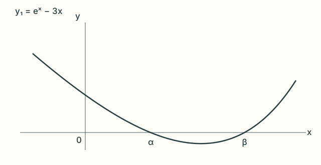
The calculator gives $\alpha\approx0.619$ and $\beta\approx1.512$ to three decimal places. Keep more digits when iterating or comparing values near a root. For the recurrence $x_{n+1}=e^{x_n}/3$, part (ii) assumes convergence. If $x_n\to L$, the shifted sequence also tends to $L$, and continuity gives

$$L=\frac13e^L\quad\Longrightarrow\quad3L=e^L \quad\Longrightarrow\quad e^L-3L=0 \quad\Longrightarrow\quad L=\alpha\ \text{or}\ L=\beta.$$

The source callout specifically explains this conditional instruction. The calculation identifies possible finite limits; it does not prove that every starting value converges. Retain the hypothesis in the concluding sentence.

For part (iii), the source calculator table displays:

A dash represents a blank cell in the source, not a zero or a failed calculation. Iterate unrounded values; repeated displayed values 0.619 do not mean exact equality with the root. The reported behaviours are increasing convergence to $\alpha$ from 0, decreasing convergence to $\alpha$ from 1, and increasing divergence from 2. The next sign analysis explains them.

Use a difference graph and preserve the relevant interval

For Example 32(iv), consider the difference asked for:

$$x_{n+1}-x_n=\frac13e^{x_n}-x_n =\frac13(e^{x_n}-3x_n).$$

The source suggests entering Y1=e^X−3X and Y2=(e^X−3X)/3. The second curve is a vertical compression of the first, retaining both roots and every sign:

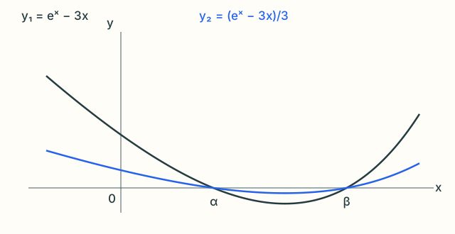
Between the roots the difference is negative; outside them it is positive:

$$\begin{aligned} \alpha<x_n<\beta&\Longrightarrow x_{n+1}-x_n<0 \Longrightarrow x_{n+1}<x_n,\\ x_n<\alpha\ \text{or}\ x_n>\beta&\Longrightarrow x_{n+1}-x_n>0 \Longrightarrow x_{n+1}>x_n. \end{aligned}$$

The source uses these graph signs. An algebraic check is $h''(x)=e^x>0$, while $h'(x)=e^x-3$ vanishes only at $x=\ln3$: the graph decreases to one minimum and then increases, giving the stated sign regions around its two roots.

For part (v), the source compares $0<\alpha$, $\alpha<1<\beta$ and $2>\beta$. To apply the sign result repeatedly, also check that later terms stay in the relevant region. The function $g(x)=e^x/3$ is strictly increasing and fixes $\alpha,\beta$, so

$$\begin{aligned} 0\le x<\alpha&\Longrightarrow x<g(x)<\alpha,\\ \alpha<x<\beta&\Longrightarrow\alpha<g(x)<x,\\ x>\beta&\Longrightarrow g(x)>x>\beta. \end{aligned}$$

Thus the sequences starting at 0 and 1 are respectively increasing/bounded above and decreasing/bounded below. Their finite limits must be $\alpha$.

The sequence starting at 2 increases and stays above $\beta$.

If it had a finite limit, that limit would be at least 2, contradicting the only possible limits in (ii); hence it is unbounded and tends to positive infinity.

This interval/boundedness reasoning supplies the detail behind the observed behaviours. Increasing alone does not imply divergence.

Relate a circle partition to AP and GP conditions

Example 33 cuts a radius-two circle into ten unequal sectors with increasing areas $a,a+d,\ldots,a+9d$. Their total equals the circle area:

$$\frac{10}{2}(2a+9d)=\pi(2)^2 \quad\Longrightarrow\quad2a+9d=\frac{4\pi}{5}.$$

The first, fourth and ninth are $a,a+3d,a+8d$. Consecutive GP ratios give

$$\begin{aligned} \frac{a+3d}{a}&=\frac{a+8d}{a+3d},\\ a^2+6ad+9d^2&=a^2+8ad,\\ 9d^2-2ad&=0,\\ d&=\frac{2a}{9}\qquad(d\ne0). \end{aligned}$$

The areas are positive and unequal, so division by $a$, $a+3d$ and $d$ is legitimate. Substitution gives $4a=4\pi/5$, hence $a=\pi/5$. The largest area is the tenth:

$$a+9d=a+2a=\frac\pi5+\frac{2\pi}{5}=\frac{3\pi}{5}\ \text{square units}.$$

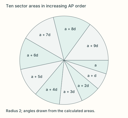
All ten labels in the source figure are retained. Its largest wedge is drawn as a quarter-circle, so treat that sketch as schematic. The calculated areas give angles $18^\circ,22^\circ,26^\circ,30^\circ,34^\circ,38^\circ,42^\circ,46^\circ,50^\circ,54^\circ$, used in this redraw. Do not infer an area from the source wedge’s apparent angle.

Compare cumulative travel distances at the same leap count

Example 34 models a jaguar chasing a white-tailed deer initially $d$ metres ahead. The deer starts with a 9 m leap and reduces each subsequent leap by 5%, so

$$D_n=\frac{9(1-0.95^n)}{1-0.95}=180(1-0.95^n).$$

As $n\to\infty$, $D_n\to180$ m. The source calls this a maximum distance. More precisely, every finite total is below 180 m and increases toward it: 180 m is the limiting upper bound, or supremum.

The jaguar starts at 6 m per leap and reduces each subsequent leap by 0.1 m, giving

$$J_n=\frac n2[12+(n-1)(-0.1)].$$

Both animals complete the same leap count in the same duration. For the initial 11 m gap, catching requires $J_n\ge D_n+11$. The source enters the difference into a calculator:

$$F(n)=\frac n2[12+(n-1)(-0.1)]-180(1-0.95^n)-11\ge0.$$

Its written table singles out:

The calculator screen also shows neighbouring counts 44–54. Computed values to four significant figures are:

The first feasible integer is 50; checking all earlier integer counts 1–49 gives negative differences. The calculation is within the physical AP range of positive jaguar leap lengths, through leap 60. Do not extend the AP into negative distances, and do not compare just the individual leap lengths instead of the cumulative travel totals.

Count bounce heights and travelled legs separately

Example 35 drops a ball from 200 cm, with each rebound height $q=8/9$ times the preceding height. The source recommends drawing a diagram, making a table and observing the pattern. Define $h_k$ as the height after rebound $k$:

The source table’s metre heading is inconsistent with the question and calculation; these values are in centimetres. The height after the kth floor contact is the kth rebound height, not the initial drop. At the fourth rebound apex, the initial descent counts once, heights 1–3 count twice and height 4 once:

$$\begin{aligned} T_4&=200+2h_1+2h_2+2h_3+h_4\\ &=200+400q+400q^2+400q^3+200q^4\\ &\approx1277.396738\ \text{cm}\approx1277\ \text{cm}. \end{aligned}$$

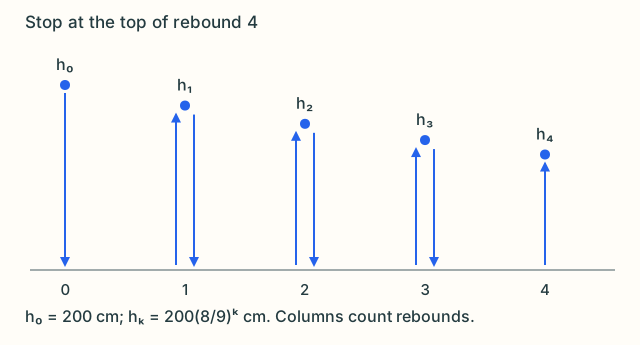
For part (ii), the first rebound below 0.01 cm satisfies the strict inequality

$$\begin{aligned} 200(8/9)^n&<0.01,\\ (8/9)^n&<0.01/200,\\ n&>\frac{\ln(0.01/200)}{\ln(8/9)}\approx84.082461. \end{aligned}$$

Dividing by the negative logarithm reverses the inequality. The least integer is 85: $h_{84}\approx0.010098$ cm is still above the threshold and $h_{85}\approx0.008976$ cm is below it.

The source totals the initial descent plus 84 completed up-and-down rebound heights:

$$\begin{aligned} T_{\mathrm{floor},85} &=200+400[(8/9)+(8/9)^2+\cdots+(8/9)^{84}]\\ &=200+400\frac{(8/9)[1-(8/9)^{84}]}{1-8/9}\\ &\approx3399.838438\ \text{cm}\approx3400\ \text{cm}. \end{aligned}$$

The lecturer notes that the final rise to the 85th apex can be omitted at the requested nearest-centimetre precision.

Its comparison screen includes both totals: adding $h_{85}$ gives $3399.847414$ cm, which also rounds to 3400 cm.

The extra ascent is small, not exactly zero.

The examiner-report note’s “initial height + 2 x other heights” describes the completed paired legs; always identify the final endpoint before deciding whether the last height is counted once or twice.

Repeated payments and the observation time

For the annual deposits in Example 36, sketch the first few years before choosing the sum. A deposit at the beginning of a year earns interest at that year’s end.

Immediately after deposit ten, the ten payments have earned 9, 8, …, 1, 0 years of interest. Thus the balance is $200(1+1.05+\cdots+1.05^9)=2515.58$ dollars to the nearest cent.

An extra multiplication by 1.05 would move the observation to the end of year ten.

Example 37 observes the other side of a repeated event: just before an injection. Write $q=e^{-1/5}$. Immediately after injection $n$, the amount is $A_n=10(1+q+\cdots+q^{n-1})$; before injection $n+1$, it is $B_n=qA_n=10(q+\cdots+q^n)$. Since $0<q<1$, the pre-injection limit is $10q/(1-q)=10/(e^{1/5}-1)\approx45.2$ units. The post-injection limit is ten units larger. The limiting behaviour is a repeating decay-and-injection cycle, not a constant amount during the day.

Check your sequence and series skills

Use the source checklist twice: after studying the lecture and again after attempting the tutorial. Its two columns are blank self-assessments, not a claim that reading a page establishes mastery. For each skill, explain the method and try a fresh example without looking at its solution.

• Distinguish finite and infinite sequences. Generate terms from $u_n=f(n)$ for the allowed positive integer indices, recover $u_1=S_1$ and $u_n=S_n-S_{n-1}$ for $n\ge2$, and describe behaviour as the index grows.
• Recognise an AP by a constant successive difference $u_{n+1}-u_n=d$. Identify its first term and finite term count; use $u_n=a+(n-1)d$. Three consecutive AP terms $u,v,w$ satisfy $2v=u+w$.
• Recognise a GP by a constant successive ratio $u_{n+1}/u_n=r$ where the denominator is nonzero. Identify its first term, ratio and finite term count; use $u_n=ar^{n-1}$. Three consecutive nonzero GP terms satisfy $v^2=uw$ and the same consecutive ratio. Keep the earlier qualifications for zero terms.
• Generate a recurrence with a calculator, describe the resulting behaviour, and express a recurrence as an explicit nth-term formula when possible.
• Distinguish finite and infinite series. Write a series in sigma notation, expand a sigma expression, and count $n-m+1$ terms from index $m$ through $n$ inclusive.
• Apply constant factors, sum/difference rules and prefix subtraction; evaluate finite sums with a calculator. Choose AP, GP or supplied square/cube-sum formulae according to the actual summand.

$$\begin{aligned} \sum_{r=m}^{n}cu_r&=c\sum_{r=m}^{n}u_r,\\ \sum_{r=m}^{n}(u_r\pm v_r)&=\sum_{r=m}^{n}u_r\pm\sum_{r=m}^{n}v_r,\\ \sum_{r=m}^{n}u_r&=\sum_{r=k}^{n}u_r-\sum_{r=k}^{m-1}u_r\quad(k<m). \end{aligned}$$

For AP sums, use $S_n=\frac n2[2a+(n-1)d]=\frac n2(a+u_n)$. For finite GP sums, use $S_n=a(1-r^n)/(1-r)=a(r^n-1)/(r-1)$ when $r\ne1$; when $r=1$, use $S_n=na$. For a nonzero infinite GP, check $|r|<1$ before using $S_\infty=a/(1-r)$.

Recognise these special sigma forms and their index endpoints:

$$\begin{aligned} \sum_{r=m}^{n}c&=(n-m+1)c,\\ \sum_{r=1}^{n}r&=\frac{n(n+1)}2,\\ \sum_{r=1}^{n}a^r&=\frac{a(1-a^n)}{1-a}=\frac{a(a^n-1)}{a-1}\quad(a\ne1). \end{aligned}$$

In the last expression, $a$ is both the first term and common ratio. For $a=1$, the sum is $n$. The finite polynomial also gives zero when $a=0$, even if a definition of GP excludes zero ratios. The Student checklist’s number-of-terms symbol is misprinted on page 58; the Teacher copy correctly uses $n$.

Choose practice by question type

The source’s page-59 routing uses lecture example, discussion-question and review-problem numbers. A dash below means the source leaves that cell blank. These are practice suggestions, not source-completion or mastery indicators.

Source correction: both copies print Examples 19, 20 and 21 under GP finite sums and leave the AP finite-sum lecture cell blank. Their actual problems use AP sums, so they belong in the AP row. Examples 24 and 25 provide GP finite-sum practice. The unchanged printed routing remains in the retained native transcription; the table above makes the correction explicit.