Worked solution
Find the largest sample meeting a strict probability bound
On average 1 in 100 light bulbs made by a factory is faulty. A sample contains n light bulbs and X counts the faulty bulbs. (i) State in context two assumptions needed for a binomial model. (ii) Require . Find the largest possible n.
CJC · Lecture · Example 4
(i) State assumptions about the bulbs
The probability that each selected bulb is faulty stays constant at 0.01, and whether a bulb is faulty is independent of whether the other bulbs are faulty. As the Teacher note emphasizes, describe independence of events or trials, not “independent probability”. When the needed binomial conditions are not supplied, make the modelling assumptions explicit.
(ii) Formula and logarithm method
Let X count faulty bulbs among n, with . Then gives , hence . Taking logs gives , so . Because , reverse the inequality when dividing: . The largest integer n is 68. The sign reversal is the distinct Teacher warning.
(ii) Calculator method and boundary evidence
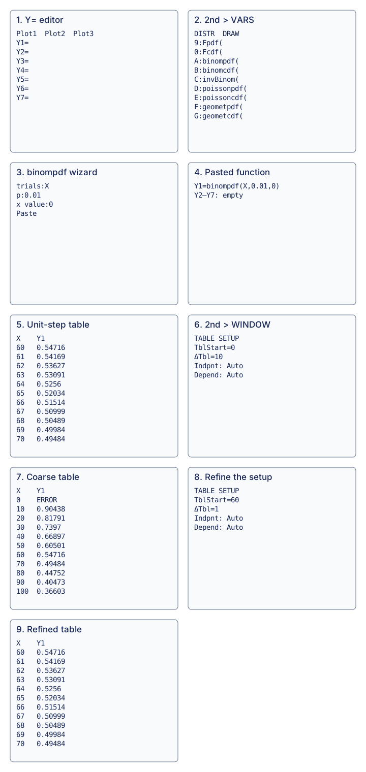
- Press Y=. 2. Press 2nd, VARS, select A:binompdf(, then ENTER. 3. Set trials:X, p:0.01, x value:0, choose Paste, then ENTER. The Y-editor contains
Y1=binompdf(X,0.01,0). Here the calculator’s X input stands for the varying trial count n. 4. Press 2nd, GRAPH and scroll to the first probability below 0.5. Present the source boundary table, as the Teacher note specifically requires:
| Sample size n | |
|---|---|
| 67 | 0.50999 |
| 68 | 0.50489 |
| 69 | 0.49984 |
At 68 the probability exceeds 0.5; at 69 it does not. Thus the largest sample is 68. For a fixed p=0.01, the no-fault probability 0.99ⁿ decreases with n, so this boundary comparison establishes the largest value.
Refine a coarse calculator search
The source continuation explains TblStart (starting value) and ΔTbl (row increment). Press 2nd, WINDOW, set TblStart=0, ΔTbl=10, with independent/dependent entries on Auto. Press 2nd, GRAPH. The table brackets the crossing between n=60 and n=70. The screenshot shows ERROR at n=0 in this calculator command; this is a calculator-domain limitation, not a claim that the mathematical zero-trial distribution is invalid. Next set TblStart=60, ΔTbl=1 through 2nd, WINDOW, then 2nd, GRAPH to locate the exact integer boundary. The full coarse and refined source tables are retained in the diagram.
Compare your sketch
Find the largest integer sample size
1. Name the varying input
The random variable counts faulty bulbs, while the calculator X below represents the sample size n. Require P(no faulty bulbs) > 0.5 with fault probability 0.01.
2. Enter the probability function
Open Y=. Through 2nd → VARS → A:binompdf(, set trials to X, p to 0.01 and x value to 0. Select Paste, then ENTER.
- Y1
- binompdf(X,0.01,0)
3. Bracket the boundary
Press 2nd → WINDOW for TABLE SETUP. Begin with TblStart=0 and ΔTbl=10, with independent and dependent entries on Auto. Open TABLE with 2nd → GRAPH; the crossing is between 60 and 70.
4. Refine to neighbouring integers
Return to TABLE SETUP. Use TblStart=60 and ΔTbl=1, then reopen TABLE.
Refine to neighbouring integers n Displayed P(no faults) 67 0.50999 68 0.50489 69 0.49984 Largest qualifying integer: n = 68
The inequality is strict: 68 qualifies and 69 does not. For this fixed model, 0.99ⁿ decreases with n. The original coarse table shows ERROR at n=0 for this calculator command; that is not a mathematical rejection of the zero-trial distribution. Full source tables remain below.
View original calculator screens
Expand diagramFit diagram to page
Use the scrollbars or arrow keys to inspect details.
Common mistakes
Reverse the inequality when dividing by a negative logarithm; show the neighboring integer probabilities.