Worked solution
Model red cars and solve a zero-or-one probability
A fixed number n of cars is observed and R counts those that are red. (i) State in context two assumptions for a binomial model. Assume now . (ii) For n=20 and p=0.15 find . (iii) For n=20 and , write an equation for p and find p numerically.
[2009/PII/11(part)]
CJC · Lecture · Example 8
(i) State the car assumptions
The probability that any one car is red stays the same throughout the sample, and the colour of each car is independent of the colours of the other cars. These are the two Teacher completions.
(ii) Convert the mixed interval
For , to 3 significant figures. The upper bound 8 is excluded; the lower bound 4 is included.
(iii) Write the equation
For , , so . This retains the complete Teacher working.
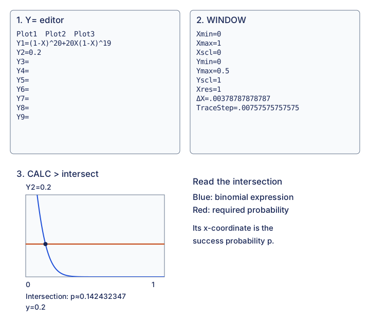
(iii) Solve with the source graph procedure
Enter the left side as Y1 and 0.2 as Y2. Adjust the window, then find the intersection; its x-coordinate is p. The source window is Xmin 0, Xmax 1, Xscl 0, Ymin 0, Ymax 0.5, Yscl 1, Xres 1 (derived ΔX≈0.003787879, TraceStep≈0.007575758). The source plot gives , hence 0.142 to 3 significant figures.
Compare your sketch
Solve for the probability that a car is red
1. Write the probability equation
Zero or one red car in 20 has probability 0.2. Add these disjoint masses to write (1−p)²⁰+20p(1−p)¹⁹=0.2.
2. Enter both sides in the Y-editor
The calculator X now stands for the unknown probability p.
- Y1
- (1-X)^20+20X(1-X)^19
- Y2
- 0.2
3. Choose a window that shows the crossing
The retained source uses these bounds. Its complete settings and plotted screens remain below.
- Xmin
- 0
- Xmax
- 1
- Ymin
- 0
- Ymax
- 0.5
4. Calculate the intersection
Press 2nd → TRACE, choose intersect, select the two curves and provide a nearby guess. Read the x-coordinate as p, not the y-coordinate.
p ≈ 0.142432347; to 3 significant figures: 0.142
Check 0 ≤ p ≤ 1. This unknown is continuous: an integer-step sample-size table is not the required numerical root solve. If asked for an equation, write it before using the calculator. Displayed intersection values are approximate.
View original calculator screens
Expand diagramFit diagram to page
Use the scrollbars or arrow keys to inspect details.
Common mistakes
For “zero or one”, add the two disjoint masses before solving for p.