Worked solution
Compare linear and squared-speed models of drag
A car is placed in a wind tunnel. Drag force at different speeds , in appropriate units, is recorded:
| 0 | 0 |
| 4 | 2.5 |
| 8 | 5.1 |
| 12 | 8.8 |
| 16 | 11.2 |
| 20 | 13.6 |
| 24 | 17.6 |
| 28 | 22.0 |
| 32 | 27.8 |
| 36 | 33.9 |
(i) Draw the scatter diagram, labelling the axes clearly.
It is thought that can be modelled by or .
(ii) Find, to 4 decimal places, the correlation coefficient between (a) and , and (b) and .
(iii) Use (i) and (ii) to explain which model is better.
(iv) Estimate when . Find a suitable regression line, use it for the estimate, and explain why neither regression of on nor of on should be used.
[N10/II/10]
CJC · Lecture · Example 11
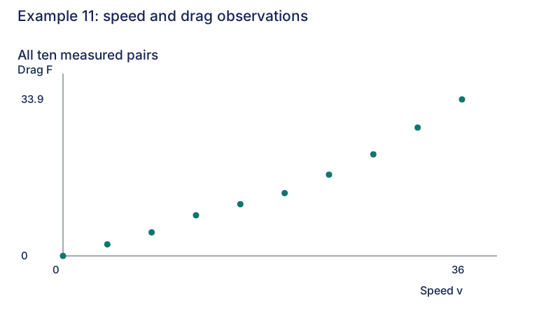
(i) Plot speed as the explanatory input
Answer
The ten observations rise with upward curvature.
The source puts in L1 and in L2, and labels axes with extrema 0,36 and 0,33.9. Preserve the origin observation as well as the other nine points. The increasing steepness suggests examining a transformed model, rather than choosing a line from correlation alone.
(ii)(a) Correlate speed and force
Answer
(4 d.p.).
Use 8:LinReg(a+bx) with Xlist=L1, Ylist=L2. The source screen gives intercept , slope , and . Retain four decimal places as requested, including the trailing zero.
(ii)(b) Generate squared speeds
Answer
(4 d.p.).
Highlight L3, press ENTER, enter L3=L1², then ENTER. The source displays squared inputs . Use Xlist=L3, Ylist=L2: calculator x represents , calculator y represents .
The printed output is , , , . Hence to 4 d.p.
(iii) Combine the scatter and coefficients
Answer
is the better of the two proposed sample models.
The source observes that drag increases at an increasing rate, and the squared-speed correlation is closer to 1 than the original-speed correlation. Both the curvature and the transformed coefficient favour the quadratic candidate. This comparison does not assert that the fitted intercept is a physically exact zero-speed drag law or establish validity beyond the measured range.
(iv) Solve the fitted response model for speed
Answer
(3 s.f.).
Speed is the prescribed explanatory variable in this wind-tunnel model, so fit force as the response to and solve that model backwards:
The source prints in the final substitution, while its preceding calculator screen gives . The final printed slope omits a digit; use the full screen coefficient, preserving this discrepancy in review. Both produce the printed final after 3-s.f. rounding. Reject the negative root because speed is nonnegative.
The blank explanation is completed from the source’s modelling convention: regressions of on or on minimise a different response error and would change the prescribed explanatory role. They are not the calibration of the fitted force model requested here.
Compare your sketch
Expand diagramFit diagram to page
Use the scrollbars or arrow keys to inspect details.
Solution notes
All ten pairs, five printed asks, original scatter, squared list, both complete regression screens and final calibration retained. The final printed squared-speed slope differs from its screen; screen coefficient used and discrepancy explicit. Explanatory-role argument is authored for the blank source explanation. No printed marks.