Worked solution
Compare tests before and after pooling two samples
A manufacturing process produces ball bearings with diameters with known standard deviation 0.04 cm. Under normal circumstances, the manufacturing process will produce ball bearings of mean diameter 0.5 cm.
(i) During a routine quality control check, a random sample of 25 ball bearings gives a mean of 0.51 cm. Is there evidence to believe that the manufacturing process is producing ball bearings of the stated diameter? Perform an appropriate test at 5% level of significance. State a necessary assumption for the test to be valid. marks
An enhancement on the manufacturing process will ensure that the diameters of the ball bearings produced are less variable.
(ii) Measurements of a sample of 100 ball bearings give the following summary statistics:
Show that the unbiased estimate of the population variance is .
Is there evidence at the 5% level of significance that after the enhancement, the manufacturing process is producing oversized ball bearings? marks
(iii) Another sample of 100 ball bearings yield the same summary statistics as the previous sample in (ii). Explain, with justification, whether the combined sample will give a different conclusion to (ii). marks
[2017/NYJC/II/9]
CJC · Review problems · Question 7
Answer
(i) , : do not reject; assume normal diameters. (ii) , : reject. (iii) pooled : reject again.
(i) Test with known population standard deviation
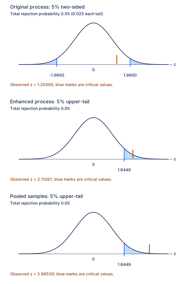
Let be an original-process bearing diameter in cm, with mean and known . Test against . Assume the population diameter distribution is normal, as required for this n 25 exact normal-mean test. Under , . Then and two-sided . Equivalently, . Do not reject: there is insufficient evidence of a departure from 0.5 cm, not proof of equality. Source Z-Test Stats input: null.5, known SD.04, sample mean.51,n 25, not-equal alternative; outputz 1.25,p.2112996779.
(ii) Estimate the enhanced-process variance
Let be an enhanced-process bearing diameter. Here and . Therefore
(ii) Test for oversized bearings, both methods
Test against , now for the enhanced population. Under , by the large-sample approximation. Using unrounded , and right-tail . Alternatively . Reject: evidence at 5% of oversized bearings. The source uses rounded , inputs estimated SD≈.02840745426, mean.506,n 100, null.5, right-tail, and displaysz 2.11210031,p.0173388734; this yields the same conclusion.
(iii) Pool the two samples
Assuming the additional sample is independent and from the same enhanced process, the pooled sample has n 200, , , and squared-deviation sum 0.1669. Thus Under , ; the right-tail statistic is and . Equivalently . Reject again: the conclusion stays the same, with stronger evidence. Source calculator inputSD≈.02832866040, mean.506,n 200, null.5, right-tail displaysz≈2.995299197,p≈.001370948. Its prose instead prints.0137; that decimal-place discrepancy is recorded below.
Compare your sketch
Expand diagramFit diagram to page
Use the scrollbars or arrow keys to inspect details.
Common mistakes
For n 25 with known SD, normality is the source’s necessary assumption; “n is large” is not the justification here.
Solution notes
Source part (i) says “n is large” and CLT despite n 25, while also stating normality; the student derivation uses that normality assumption. Source critical 1.6445 should be 1.644853627. In(iii), calculatorp≈.001370948 but prosep=.0137; correct decimal placement and both source versions retained. Variable X/Y slips are reconciled to the enhanced-process variable.