Worked solution
Audit the sampling frame and a frequency-table test
(a) College students intending to further their studies overseas have to sit for a mandatory Overseas Universities Test (OUT). Researcher Mr Anand wishes to find out if male college students tend to score higher for OUT compared to female college students.
Mr Anand’s colleague randomly selects 150 male and 150 female students from the combined student population of three particular colleges near his home to form a sample of 300 college students for the research.
Explain whether this sample is a random sample. marks
(b) The mean OUT score for all college students in 2016 is 66. Mr Anand randomly selects 240 college students taking OUT in 2017 and their scores, , are summarised in the following table:
| Score, | 60 | 65 | 68 | 70 | 75 | 80 |
|---|---|---|---|---|---|---|
| Frequency, | 40 | 90 | 63 | 27 | 18 | 2 |
(i) Write down the unbiased estimates of the population mean and variance of the OUT scores for the college students in 2017. mark
(ii) Test, at the 10% level of significance, whether the mean OUT score for all college students in 2017 is higher than the mean score attained in 2016. marks
(iii) Explain what is meant by the phrase “10% level of significance” in this context. mark
(iv) Mr Anand draws a new sample of 240 male college students. Using the unbiased estimate for the population variance computed in (i), find the range of values for the sample mean that is required for this new sample to achieve a different conclusion from that in (ii). marks
[2017/TJC/II/10]
CJC · Review problems · Question 8
Answer
Table estimates: , . : reject at 10%. New-sample non-rejection requires using that variance.
(a) Sampling-frame limitation
The sample is not a simple random sample of all college students: those outside the three nearby colleges have zero chance of inclusion. Random selection within the chosen colleges does not remove that coverage bias. The source calls the sample non-random/biased for this reason.
(b)(i) Frequency-table estimates and calculator workflow
Enter scores in one list and frequencies in a second, then run 1-Var Stats with the frequency list. The source screen shows n 240, , , , and unbiased sample SD . Direct calculation gives Thus the mean is 66.4 and variance 16.9 to 3 s.f. The source prose truncates the mean to 66.391 and SD to 4.1048, then gives variance 16.849≈16.8; those are premature-rounding differences from its own screen and original table.
(b)(ii) P-value and critical-value methods
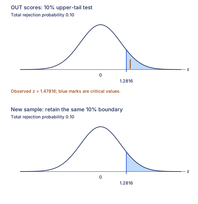
Let be the population mean 2017 OUT score. Test against . For the random n 240 sample, under , . Retaining table precision gives and upper-tail . Equivalently . Reject: sufficient evidence at 10% of a higher mean. Source Z-Test uses roundedSD 4.1048, mean 66.391,n 240, null 66, right-tail; its z≈1.475673834 and p≈.0700157709 lead to the same decision.
(b)(iii) State the conditional error probability
If the true population mean 2017 score is 66, this 10% upper-tail procedure has probability 0.10 of rejecting that null and wrongly concluding that the mean exceeds 66. This is a Type I error probability under the null, not a 10% probability that this particular conclusion is wrong.
(b)(iv) Reverse the test decision
For the new sample of male students, apply the requested variance from (i) and null reference 66 to that population. A different conclusion means not rejecting. Using the convention reject for , Hence . The source’s is a rounded boundary, not an exact real-valued set. With its rounded variance 16.849, the boundary is slightly smaller but still about 66.3396. Inference from the new sample concerns male students, not automatically all students.
Compare your sketch
Expand diagramFit diagram to page
Use the scrollbars or arrow keys to inspect details.
Common mistakes
Do not round the test boundary to 66.3 before classifying a new mean; Type I error is conditional on the null hypothesis.
Solution notes
Source 1-Var Stats screen retains the correct table mean and SD; prose truncations cause its 16.849/16.8 variance and.0700 p-value. Correct retained-precision results are shown alongside them. Source critical-method heading says 5% instead of 10% and its sketch labelz 2.11 conflicts with its own computedz 1.48; the diagram here uses the actual test.