Solve a normal interval condition and assess the model

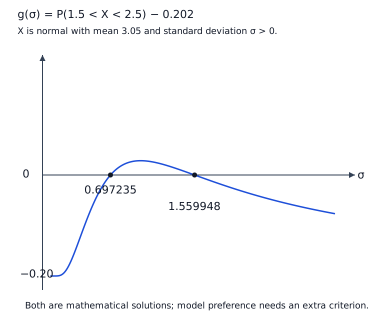
For $X\sim N(3.05,\sigma^2)$, solve $\Phi[(2.5-3.05)/\sigma]-\Phi[(1.5-3.05)/\sigma]=0.202$ for $\sigma>0$. The source plots this probability minus 0.202 against $\sigma$. The roots are approximately 0.697235 and 1.559948, hence $\sigma=0.70$ kg or 1.56 kg to 2 dp.

Using the printed rounded values, the source finds about 70% in the normal-weight category for $\sigma=0.70$ versus 37% for $\sigma=1.56$. It rejects 1.56 because this would make the outside categories collectively more likely. Its alternative reason is a negative-weight probability of about 0.03 for 1.56 versus about $6.6\times10^{-6}$ for 0.70. Both roots solve the stated interval equation; preferring the smaller one uses an additional modelling-plausibility criterion. Neither positive-variance normal model literally excludes all negative weights.

Now use the explicitly imposed $\sigma=0.86$, not the value chosen in(i). For $Y\sim N(2.8,0.86^2)$, the outside-category probability is $1-P(2.5<Y<4)\approx1-0.55493$. Assuming independent birth weights, the requested probability is $[1-P(2.5<Y<4)]^3\approx0.0882$.

Let independent $X_1,X_2\sim N(3.05,0.86^2)$ and $Y\sim N(2.8,0.86^2)$. For $A=(X_1+X_2)/2-2Y$, the mean is $3.05-2(2.8)=-2.55$ and variance is $0.5^2(2\cdot0.86^2)+2^2(0.86^2)=3.3282$. Thus $A\sim N(-2.55,3.3282)$ and $P(|A|<2)=P(-2<A<2)\approx0.375$.

For independent identically distributed costs with mean 2800 and variance $500^2$, the CLT gives $\bar W\mathrel{\dot\sim}N(2800,500^2/50)=N(2800,5000)$. Hence $P(\bar W>3000)\approx0.00234$.