Correlation and linear regression
Choose the response and fit a line · Diagrams · Complete reading
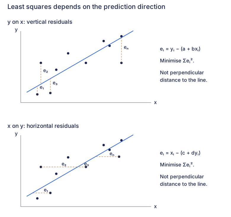
Two regression directions
Compare the fitted response on the same x-horizontal and y-vertical axes. These source-role sketches preserve illustrative points and lines, not numerical observations or regressions calculated from the drawing.
Weak linear association
- Solid: y on x
- Dashed: x on y
Strong linear association
- Solid: y on x
- Dashed: x on y
Keep the two response models distinct
The y-on-x fit minimises squared vertical residuals; the x-on-y fit minimises squared horizontal residuals on these axes. Rearranging one fitted equation does not generally produce the other fitted regression.
Both fitted lines pass through the means
For paired data with both variables varying, both least-squares regressions pass through this mean point. Use the actual observations or fitted equations to find it; the schematic positions supply no numerical mean.
At exactly zero linear correlation
When both variables vary and r is zero, both regression coefficients are zero. On the same axes, y-on-x is horizontal and x-on-y is vertical. The vertical line cannot be rewritten as a single-valued function y of x.
- Use the same axes and scale when comparing the two directions. A drawn angle is not a scale-independent measure of correlation; rescaling an axis changes the angle. Do not read a numerical r from these sketches.
- With perfect linear association and both variables varying, the fitted lines coincide. A constant variable makes the usual correlation coefficient undefined, rather than providing a zero-correlation example.
- Choosing a regression for prediction still depends on the prescribed explanatory role. Use the linked method to distinguish direct prediction from inverse calibration.
- Zero linear correlation does not rule out a nonlinear relationship. Inspect the scatter before accepting a line.
Compare with the source direction sketches
Expand diagramFit diagram to page
Use the scrollbars or arrow keys to inspect details.
Vertical and horizontal residuals
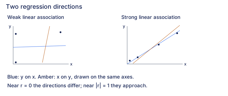
Choose the response before measuring a residual. Both sketches keep x horizontal and y vertical. Their point positions and lines are schematic; they are not numerical data or fits calculated from those positions.
y on x: vertical residuals
Predict y from x
Keep the observed x coordinate fixed. The line supplies the predicted y response at that same input.
Measure the vertical residual
The residual is observed y minus predicted y. It is signed; the dashed segment shows its magnitude along the response coordinate.
Minimise squared vertical residuals
Choose a and b to minimise this sum over every observation. Squaring prevents positive and negative residuals from cancelling. The drawing marks four residual roles, not only four terms in the sum.
Compare each observation with its prediction.
- Ringed point: e₁.
e₁: below its prediction
The ringed observation lies below its prediction, so observed y minus predicted y is negative.
- Ringed point: e₂.
e₂: above its prediction
The ringed observation lies above its prediction, so observed y minus predicted y is positive.
- Ringed point: e₃.
e₃: below its prediction
The ringed observation lies below its prediction, so observed y minus predicted y is negative.
- Ringed point: eₙ.
eₙ: below its prediction
The ringed observation lies below its prediction, so observed y minus predicted y is negative.
x on y: horizontal residuals
Predict x from y
Keep the observed y coordinate fixed. The line supplies the predicted x response at that same input.
Measure the horizontal residual
The residual is observed x minus predicted x. It is signed; the dashed segment shows its magnitude along the response coordinate.
Minimise squared horizontal residuals
Choose c and d to minimise this sum over every observation. Squaring prevents positive and negative residuals from cancelling. The drawing marks four residual roles, not only four terms in the sum.
Compare each observation with its prediction.
- Ringed point: e₁.
e₁: right of its prediction
The ringed observation lies right of its prediction, so observed x minus predicted x is positive.
- Ringed point: e₂.
e₂: left of its prediction
The ringed observation lies left of its prediction, so observed x minus predicted x is negative.
- Ringed point: e₃.
e₃: right of its prediction
The ringed observation lies right of its prediction, so observed x minus predicted x is positive.
- Ringed point: eₙ.
eₙ: right of its prediction
The ringed observation lies right of its prediction, so observed x minus predicted x is positive.
- Changing the response changes the least-squares problem. Rearranging one fitted equation does not generally give the other fitted regression.
- Measure along the response coordinate, not perpendicular to the line. A residual may be positive, negative or zero; its square is nonnegative.
- The two source panels have distinct schematic observations. Do not treat them as numerical fits of one shared dataset, or calculate coefficients or residual totals from their drawing coordinates.
- The two sums measure errors in different response coordinates and may have different units. Compare candidate fits for the same response on the same observations; do not rank y-on-x against x-on-y by their raw residual totals.
Compare with the source residual sketches
Expand diagramFit diagram to page
Use the scrollbars or arrow keys to inspect details.