Discrete random variables

A random variable assigns a numerical value to each outcome. A discrete distribution has nonnegative probabilities summing to 1. Its expectation is $E(X)=\sum xp(x)$ and variance is $E(X^2)-[E(X)]^2$. A linear transformation gives E(aX+b)=aE(X)+b and Var(aX+b)=a²Var(X).

From outcomes to a numerical random variable

The source outline covers discrete random variables, probability distributions, expectations and variances. A random variable is a function assigning one real number to each outcome in a sample space. Capital letters such as $X$ denote random variables; lowercase $x$ denotes an observed value. In the source example, $X_1$ and $X_2$ represent two independent repetitions of the three-toss experiment. Subscripts are labels; they do not by themselves imply independence.

For three coin tosses the complete sample space is $S=\{HHH,HHT,HTH,THH,HTT,THT,TTH,TTT\}$, where H means heads and T means tails. Let $X$ count heads, assigning the values $3,2,2,2,1,1,1,0$ respectively. The Teacher note asks us to explain fair: heads and tails each have probability $1/2$ on an individual toss. With independent tosses, all eight sequences have probability $1/8$; independence is a separate modelling assumption.

A discrete random variable takes finitely many or at most countably infinitely many values. Draw two balls successively without replacement from four red and three black balls, and let X count reds:

Colour outcome	RR	RB	BR	BB
Red count x	2	1	1	0

R means a red ball was drawn and B means a black ball. Different outcomes can have the same numerical value; these four colour strings need not be equally likely.

Throw a fair die until the first six. Here T means a six and F means a non-six (different notation from the coin example):

Stopped outcome	T	FT	FFT	FFFT	…
Number of throws y	1	2	3	4	…

Under independent throws the die eventually gives a six with probability one. The source lists the finite stopped outcomes; the never-six sequence is a null event, not a finite waiting time. Discrete values need not be integers: the source’s shoe-size example includes $8\frac12$.

Probability mass functions

Each possible value is assigned a probability. The source calls the formula a probability function, probability mass function or probability distribution (and later “probability distribution function”). We use mass function $f(x)=P(X=x)$ to distinguish it from the cumulative function $P(X\le x)$. As emphasized in the source’s Function note, the input is a numerical value and the output is its probability. A valid law satisfies $0\le f(x)\le1$ and $\sum_xf(x)=1$, summed over all possible values.

For the number of heads in three independent fair tosses:

x	0	1	2	3
$P(X=x)$	$1/8$	$3/8$	$3/8$	$1/8$

Equivalently $f(x)=\binom3x(\frac12)^3$ for $x=0,1,2,3$, and zero elsewhere. The middle values combine three sequences each; they are not equally likely to the endpoints. Always check nonnegativity and total probability one before using a distribution.

Descriptive statistics: centre and spread

Mean, median and mode describe central tendency. Standard deviation measures spread; variance is its square and measures variability. Together these provide a descriptive summary rather than a complete account of a data set.

For an observed data list, the mode is the value occurring most often. Sort the observations in ascending or descending order to find the median: the middle observation for an odd count, or the average of the two middle observations for an even count. The source examples are:

Data	Mode	Median
1, 3, 3, 6, 7, 8, 9	3	6
1, 2, 3, 4, 5, 6, 6, 9	6	$(4+5)/2=4.5$
1, 1, 1, 3, 4, 6, 8, 8, 8	1 and 8	4

For a discrete probability distribution, a mode maximizes $P(X=x)$. A median $m$ satisfies both $P(X\le m)\ge0.5$ and $P(X\ge m)\ge0.5$.

Qualify the printed parity shortcut. The source also prints $m=(m_1+m_2)/2$ for an even number of values, with $P(X\le m_1)\ge0.5$ and $P(X\ge m_2)\ge0.5$, and $m=m_1=m_2$ for an odd number.

Counting observations works for an empirical data list; counting distinct possible values of a non-uniform distribution does not determine its median. Use the two probability inequalities.

Example 7 has five possible values, yet its source answer is the midpoint $3.5$ of the full median interval $[3,4]$.

When cumulative probability is exactly one half across a gap, the midpoint is a reporting convention, not the sole mathematical median.

Mean as a weighted long-run average

For data $x_1,x_2,\ldots,x_n$, $\bar x=(x_1+x_2+\cdots+x_n)/n$. For a random variable with mass function $f(x)$, its mean or expectation is $\mu=E(X)=\sum_xxf(x)$. With independent repetitions under a fixed distribution and a finite expectation, this is the long-run average interpretation. Infinite distributions require the appropriate convergence; symmetry alone does not guarantee an expectation exists.

The source scores one fair coin throw as $0$ for heads and $1$ for tails:

x	0	1
$P(X=x)$	$1/2$	$1/2$

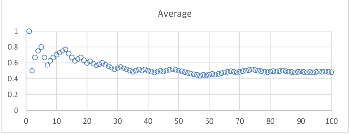
Repeat the experiment n times and plot the running average.

The Student copy provides blank axes; the Teacher copy completes one particular run, reproduced in the diagram below.

Its horizontal axis covers 0–100 tosses and its vertical average covers 0–1. The early averages fluctuate and later values settle near $1/2$.

This one run illustrates the long-run mean $E(X)=0(1/2)+1(1/2)=1/2$; it is not a claim that every run approaches monotonically or equals one half after a fixed number of tosses.

Constant and symmetric distributions: source proofs

If a is constant, its distribution places probability one at a:

x	a
$P(X=x)$	1

Therefore $E(a)=a(1)=a$.

For a finite distribution symmetric about $x=a$, let $Y=X-a$. Then $P(Y=y)=P(Y=-y)$. With $2n+1$ listed values, write them as $-y_n,-y_{n-1},\ldots,-y_1,0,y_1,\ldots,y_{n-1},y_n$. Expanding the source sum gives

$E(Y)=[-y_nP(Y=-y_n)]+[-y_{n-1}P(Y=-y_{n-1})]+\cdots+[-y_1P(Y=-y_1)]+0P(Y=0)+[y_1P(Y=y_1)]+\cdots+[y_{n-1}P(Y=y_{n-1})]+[y_nP(Y=y_n)].$

Replace each negative-side probability by its equal positive-side probability. Every pair becomes $-y_iP(Y=y_i)+y_iP(Y=y_i)=0$, and the central term is zero, so $E(Y)=0$. Since $X=Y+a$, shifting every value back by a gives $E(X)=0+a=a$. If only $2n$ values are listed, insert the central value a with probability zero; the same cancellation applies. Follow the Teacher suggestion to use Example 8 to see the matching pairs explicitly.

Expectation of a function

For $Y=g(X)$ and mass function $f(x)$, $E(Y)=E[g(X)]=\sum_xg(x)f(x)$, whenever the expectation exists. You may average g(x) using X’s masses without first constructing a separate Y table.

The source proof begins with n possible values:

x	$x_1$	$x_2$	$x_3$	…	$x_n$
$P(X=x)$	$p_1$	$p_2$	$p_3$	…	$p_n$
$y=g(x)$	$y_1$	$y_2$	$y_3$	…	$y_n$

Qualify the printed proof. Its assertion $P(Y=y_i)=P(X=x_i)=f(x_i)$ is valid when each image $y_i$ has just one preimage among the possible X values. Under that one-to-one condition, its full chain is $E(Y)=\sum_{i=1}^ny_iP(Y=y_i)=\sum_{i=1}^ng(x_i)P(X=x_i)=\sum_{i=1}^ng(x_i)f(x_i)=\sum_xg(x)f(x)$.

For a general transformation the images may repeat, as in Example 5. Group first: $P(Y=z)=\sum_{i:g(x_i)=z}p_i$. Then $E(Y)=\sum_zz\sum_{i:g(x_i)=z}p_i=\sum_ig(x_i)p_i$. This proves the same rule without the extra one-to-one restriction, while the original printed proof remains in the native transcription.

Variance describes spread around the mean

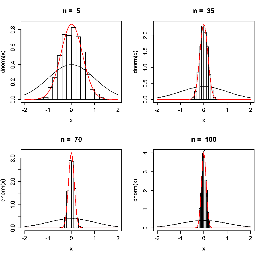
A mean locates the centre but does not describe the full shape or spread. The source’s four panels, labelled n=5,35,70,100, are reproduced below with their original histograms, red and black curves, x axes and different vertical scales. They are centred at zero but have different spreads. Compare horizontal concentration; the varying height scales are not a common probability scale. Source attribution printed in the PDF: University of Pennsylvania illustration.

For a discrete X with mean $\mu$, the variance is the probability-weighted average squared distance from that mean:

$\sigma^2=\operatorname{Var}(X)=E[(X-\mu)^2]=\sum_x(x-\mu)^2f(x).$

The standard deviation is $\sigma=\sqrt{\operatorname{Var}(X)}$, taking the nonnegative square root. The source says “positive”; zero variance has standard deviation zero. These finite formulas apply when the second moment is finite.

The source’s alternative formula is $\operatorname{Var}(X)=E(X^2)-[E(X)]^2$. Retain every step of the proof:

$$\begin{aligned} \sigma^2&=\sum_x(x-\mu)^2f(x)\\ &=\sum_x(x^2-2\mu x+\mu^2)f(x)\\ &=\sum_xx^2f(x)-\sum_x2\mu xf(x)+\sum_x\mu^2f(x)\\ &=\sum_xx^2f(x)-2\mu\sum_xxf(x)+\mu^2\sum_xf(x)\\ &=E(X^2)-2\mu^2+\mu^2\\ &=E(X^2)-\mu^2\\ &=E(X^2)-[E(X)]^2. \end{aligned}$$

The three sums in the fourth line are respectively $E(X^2)$, $\mu$ and $1$. Constants have no variability: a variable equal to a with probability one has the one-column table $x=a$, $P(X=x)=1$; $E(a)=a(1)=a$ and $\operatorname{Var}(a)=(a-a)^2(1)=0$. The source points ahead to Section 5, the appendix relating these probability-weighted formulas to the mean and variance of a frequency distribution from secondary school; use that connection to recognize the same weighted-average structure.

Linear transformations: complete source proofs

For constants a and b, if $E(X)=\mu$ and $\operatorname{Var}(X)=\sigma^2$, then $E(aX\pm b)=aE(X)\pm b$ and $\operatorname{Var}(aX\pm b)=a^2\operatorname{Var}(X)$. The same choice of plus or minus is used throughout each expression. For discrete X with mass f(x), retain the expectation proof:

$$\begin{aligned} E(aX\pm b)&=\sum_x(ax\pm b)f(x)\\ &=\sum_x[axf(x)\pm bf(x)]\\ &=\sum_xaxf(x)\pm\sum_xbf(x)\\ &=a\sum_xxf(x)\pm b\sum_xf(x)\\ &=aE(X)\pm b\\ &=a\mu\pm b. \end{aligned}$$

The last two sums are E(X) and 1 respectively. The variance proof uses that transformed mean:

$$\begin{aligned} \operatorname{Var}(aX\pm b)&=E[\{(aX\pm b)-(a\mu\pm b)\}^2]\\ &=E[(aX-a\mu)^2]\\ &=\sum_x(ax-a\mu)^2f(x)\\ &=\sum_xa^2(x-\mu)^2f(x)\\ &=a^2\sum_x(x-\mu)^2f(x)\\ &=a^2\operatorname{Var}(X)\\ &=a^2\sigma^2. \end{aligned}$$

The sum of squared deviations is Var(X). Adding or subtracting b cancels inside the deviation; scaling by a squares the distance multiplier. The standard deviation therefore scales by $|a|$, a supplementary consequence that also handles negative a.

Calculator values: population spread and stored precision

The full seven-step Example 11 workflow enters probabilities as frequency weights. Use the population output σx and square its stored value to obtain variance. The source’s n=1 is the sum of those weights. Do not substitute the sample output Sx or retype a rounded sigma. Example 13 uses the same workflow before applying the transformation rules.

Independent observations and repeated trials

The source models an experiment repeated n times under identical conditions, such as repeated fair-die throws. X denotes one result and $X_1,\ldots,X_n$ the respective first through nth results. They are modelled as independent and identically distributed observations of X. Identical conditions justify a common distribution in this model; independence is a separate assumption, not a consequence of the subscripts or the phrase “identical conditions”.

For n independent observations with the same finite moments, the source gives

$$E(X_1\pm X_2\pm\cdots\pm X_n)=E(X_1)\pm E(X_2)\pm\cdots\pm E(X_n),$$

and

$$\operatorname{Var}(X_1\pm X_2\pm\cdots\pm X_n)=\operatorname{Var}(X_1)+\operatorname{Var}(X_2)+\cdots+\operatorname{Var}(X_n)=n\operatorname{Var}(X).$$

The signs carry through the expectation, but all variance contributions are added. The source omits proofs because they use joint distributions and covariance, which it identifies as outside the syllabus.

Read the dependence remark as a restriction on using a rule. Even without independence, $E(X\pm Y)=E(X)\pm E(Y)$. The source prints $\operatorname{Var}(X\pm Y)\ne\operatorname{Var}(X)+\operatorname{Var}(Y)$ for dependent variables. The precise statement is that adding their variances is not guaranteed; some dependent pairs can still have additive variances. The equality alone does not establish independence; its failure rules out independence when these variances exist.

Doubling one observation versus adding two independent observations

For two independent copies of X:

Quantity	Double one observation	Add two independent observations
Expectation	$E(2X)=2E(X)$	$E(X_1+X_2)=E(X_1)+E(X_2)=2E(X)$
Variance	$\operatorname{Var}(2X)=2^2\operatorname{Var}(X)$	$\operatorname{Var}(X_1+X_2)=\operatorname{Var}(X_1)+\operatorname{Var}(X_2)=2\operatorname{Var}(X)$

The source warning $2X\ne X_1+X_2$ means these constructions are not interchangeable in general. With positive variance, their variances differ by a factor of two; a constant zero-variance case is a degenerate exception. Example 14 connects normalization and base moments to a transformation and an independent sum. Example 15 makes the independent outcome table explicit before comparing signed and absolute differences.

Appendix: from observed frequencies to a probability law

A fair die is tossed 20 times. The source data, in their original order, are:

5, 4, 5, 3, 6, 2, 1, 1, 6, 3, 3, 1, 6, 5, 1, 3, 2, 1, 3, 5.

(i) Find the mean and variance of this set of data. Method 1: use frequencies. Here $f(x)$ denotes an observed frequency, rather than the probability-mass-function notation used earlier. Write $n=20$ and $\bar x=\sum_x xf(x)/n$.

$$\bar x=\frac{1(5)+2(2)+3(5)+4(1)+5(4)+6(3)}{20}=\frac{66}{20}=3.3.$$

Score $x$	Frequency	Relative frequency	$(x-\bar x)^2$
1	5	$5/20=0.25$	$(1-3.3)^2=5.29$
2	2	$2/20=0.1$	$(2-3.3)^2=1.69$
3	5	$5/20=0.25$	$(3-3.3)^2=0.09$
4	1	$1/20=0.05$	$(4-3.3)^2=0.49$
5	4	$4/20=0.2$	$(5-3.3)^2=2.89$
6	3	$3/20=0.15$	$(6-3.3)^2=7.29$

The source uses the variance with divisor n, not the unbiased sample-variance estimator with divisor n−1:

$$v=\frac{\sum_x(x-\bar x)^2f(x)}{n}=\frac{(1-3.3)^2(5)+(2-3.3)^2(2)+(3-3.3)^2(5)+(4-3.3)^2(1)+(5-3.3)^2(4)+(6-3.3)^2(3)}{20}.$$

Equivalently, $v=(5.29)(0.25)+(1.69)(0.1)+(0.09)(0.25)+(0.49)(0.05)+(2.89)(0.2)+(7.29)(0.15)=3.21$.

Method 2: use relative frequencies as an empirical probability distribution. Let $X_{\rm emp}$ be a value selected uniformly from these 20 recorded observations, so repeated scores receive their observed relative frequencies:

$x$	1	2	3	4	5	6
Empirical probability	$5/20$	$2/20$	$5/20$	$1/20$	$4/20$	$3/20$

$$E(X_{\rm emp})=1(5/20)+2(2/20)+3(5/20)+4(1/20)+5(4/20)+6(3/20)=3.3.$$ $$E(X_{\rm emp}^2)=1^2(5/20)+2^2(2/20)+3^2(5/20)+4^2(1/20)+5^2(4/20)+6^2(3/20)=141/10.$$

Therefore $\operatorname{Var}(X_{\rm emp})=E(X_{\rm emp}^2)-[E(X_{\rm emp})]^2=14.1-3.3^2=3.21$.

(ii) What happens to relative frequencies after many tosses, for example 10,000? Under repeated independent fair-die tosses, the relative frequency for each face approaches $1/6$ in the long-run probability model. This does not say all six counts are exactly equal after a particular finite number of tosses, or that each new toss makes the approximation better.

(iii) Connect the data calculation to expectation and variance. As n grows, the sample mean approaches the theoretical fair-die mean:

$$1(1/6)+2(1/6)+3(1/6)+4(1/6)+5(1/6)+6(1/6)=\sum_x xP(X=x)=7/2.$$

This is the sense in which the source calls expectation a limiting value of sample means. The population variance uses $\mu=E(X)$:

$$\operatorname{Var}(X)=\sum_x(x-\mu)^2P(X=x)=35/12.$$

The source’s last line writes $\bar x$ inside a variance sum weighted by the theoretical probabilities. Read this as a limiting connection: the empirical variance is $\sum_x(x-\bar x)^2f(x)/n$, while the theoretical variance is centred at $\mu$. The empirical values 3.3 and 3.21 from these 20 observations are not the true fair-die moments $7/2$ and $35/12$. Both original copies are retained with the printed notation unchanged.