Hypothesis tests for a mean
← Back to learning units · Complete chapter reading and print view · Open reference notes separately
By the end, you can
- Formulate hypotheses before examining a result
- Choose one-sided or two-sided evidence
- Interpret p-values and conclusions in context
about 30 minutes for the lesson · practise at your own pace.
The central idea
A test asks how unusual the observed statistic would be if the null model were true. State H₀, H₁ and significance level first. For a normal population with known variance, the standardised sample mean uses . A p-value measures a tail probability under H₀, not the probability that H₀ is true.
Organise a z-test around the claim
The source’s eight steps are: define X and population mean μ; state the distributions of X and the sample mean under (including CLT justification if needed); state hypotheses; state the test statistic; state α; specify rejection using a p-value or critical value; calculate; conclude in context.
Its scenario assumes normal masses with variance , samples 100 men and observes mean 77.2 kg. The claim “more than 75 kg” at 5% gives , and under , with an upper-tail test.
Here is the hypothesised population mean, not the observed sample mean 77.2; the source paragraph calling μ₀ a sample mean is inaccurate. A test assesses how unusual the observation is under the null model, not the probability that is true. The full mass scenario is worked below; the later examples below apply the large-sample approximation and reverse test decisions to find unknowns.
Why take a sample?
The source contrasts testing a whole population with drawing a practical sample. Its introductory contexts are mean filtration efficiency in product-quality checks and a school mean-height claim of 1.6 metres assessed with a sample of 50 students.
A sample can supply evidence about a population parameter while leaving uncertainty; it cannot prove or disprove a claim with certainty.
The source also lists one-sample, two-sample and paired t-tests, ANOVA and chi-squared tests as examples of other test families. This chapter concentrates on a population mean using a z-test, with the exact or approximate reference model justified for the case.
Critical regions: allocate the significance level
Expand diagramFit diagram to page
Use the scrollbars or arrow keys to inspect details.
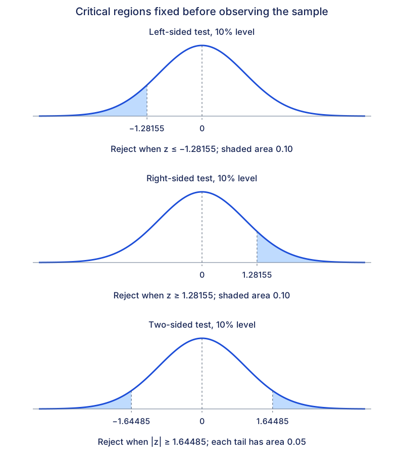
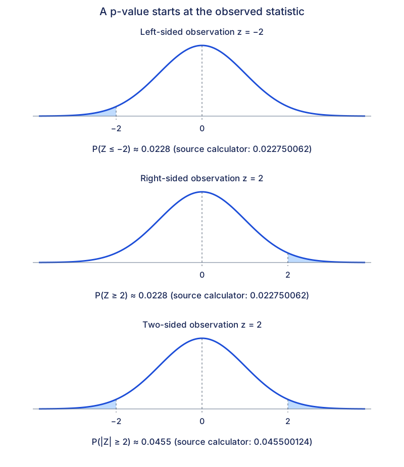
Observed tail probabilities
Expand diagramFit diagram to page
Use the scrollbars or arrow keys to inspect details.
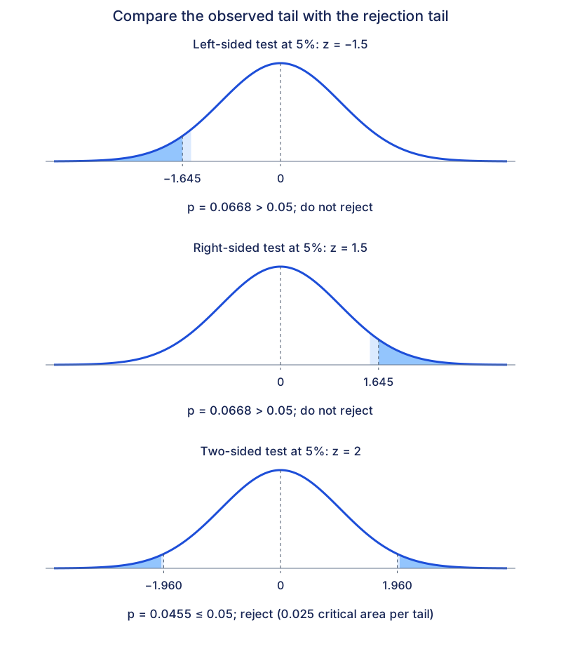
Compare p-values and critical values at 5%
Expand diagramFit diagram to page
Use the scrollbars or arrow keys to inspect details.
Explore
Use the three 5% decisions above. Before calculating again, predict which decisions could change at 1%. For a two-sided test, sketch the rejection tails at both levels on the same standard normal curve. Explain why the observed statistic and its p-value stay fixed while the critical values move.
Worked example
A machine is intended to fill bottles to a population mean of 500 ml. Independent fills are normally distributed with known standard deviation 8 ml. A random sample of 16 bottles has mean 504 ml. Before taking the sample, the inspector chose a 5% test for an increase.
Define as the mean fill volume and state , . Under , exactly.
The standard error is 2 ml, so the observed .
The upper-tail probability is approximately 0.0228. Reject at 5%: there is evidence that the population mean fill exceeds 500 ml.
The test concerns the mean, not whether every bottle exceeds 500 ml.
A p-value is calculated under the null model. It is neither the probability that the claim is true nor a measure of the practical size of the difference.
Check your understanding
A supplier claims that the population mean lifetime of its lamps is 1200 hours. An inspector suspects a decrease and chooses a 5% test before collecting data. Lifetimes are normally distributed with known standard deviation 80 hours; 25 independent randomly selected lamps have mean lifetime 1176 hours. Set up and carry out the test, explain the p-value in context, and state what the conclusion can and cannot establish.
Let be the population mean lamp lifetime in hours. Use , . Under , exactly.
The standard error is 16 hours and the observed statistic is .
The left-tail , so do not reject at 5%.
If the claimed mean and model were correct, a sample mean at most 1176 hours would occur with probability about 0.0668.
There is insufficient evidence of a decrease; this does not prove that the mean is 1200 hours.
Mastery learning objectives
At the end of this chapter, I should be able to:
Choose a practice question
The following nine rows retain the printed source map and its question references. A dash means the source cell is blank. The qualifications below identify misplaced references; the linked Discussion and Review sets retain their own reviewed wording.
| Common question type | Lecture examples | Discussion | Review follow-up |
|---|---|---|---|
| Explain significance or p-value in context | — | 1(ii), 5, 7(iv) | 6(ii), 9(b)(iii) |
| Explain whether a sample is random | — | — | 9(a) |
| Compare one-tailed and two-tailed conclusions | — | 4(a)(b) | 7(iii) |
| Test a normal-population mean using z | 1, 2, 5(i) | 1(i) | — |
| Test a non-normal-population mean using a large sample and CLT | 3 | 2, 4(1st part), 5, 7(i)(ii), 8(i)(ii) | 1(i), 4, 6, 8, 9(b)(i)(ii), 10(iv) |
| Find unknown significance using p | 4 | 7(iii) | 3 |
| Find unknown reference mean using critical values | 5(ii) | 6 | 2, 5 |
| Find unknown observed mean using critical values | 6(i)(ii) | 3, 8(iii) | 7(i)(ii), 9(b)(iv), 10(v) |
| Find unknown n using critical values | 6(iii) | 1(iii) | 1(ii) |
Source-map qualifications: Example 5(i) is printed in the normal-population row, but its cereal population is not stated normal; its large n=80 working uses CLT.
The printed Review 9(a)/9(b) labels do not occur on the current Review 9, which is the virologist question with parts (i)–(v).
For the OUT sampling-frame and score questions use Review 8(a), 8(b)(i)–(iv).
For a one-sided deduction from two-sided rejection use Review 6(iii); printed Review 7(iii) instead pools bearing samples.
Review 6(ii), printed in the p-value-meaning row, asks for waiting-mean bounds; Review 5’s final ask explicitly requests a contextual p-value explanation. These source references are retained rather than silently renumbered.
Practice questions
Practice section 1 · Questions 1–6
Assess Alice’s claim about mean mass · Turn three claims into hypotheses · +4 more
Practice section 2 · Questions 7–12
Test cereal mass and invert a two-sided rejection · Reverse a known-variance test for mean time and sample size · +4 more
- Test cereal mass and invert a two-sided rejection
- Reverse a known-variance test for mean time and sample size
- Test the claimed bulb power and change the sample size
- Test a longer-life bulb claim using CLT
- Find the spending rejection boundary without over-rounding
- Test standby time and compare significance statements
Practice section 3 · Questions 13–18
Pool battery samples before calculating a test · Find the reference means rejected by an upper-tail test · +4 more
- Pool battery samples before calculating a test
- Find the reference means rejected by an upper-tail test
- Distinguish unbiased variance, estimated SD and significance
- Test a minimum string length and interpret a strict boundary
- Test a revision-time claim and find a minimum sample size
- Invert a two-sided test without imposing integer means
Practice section 4 · Questions 19–24
Find significance levels that reject a wage claim · Test a filling machine using a sample standard deviation · +4 more
- Find significance levels that reject a wage claim
- Test a filling machine using a sample standard deviation
- Interpret an upper-tail p-value in context
- Deduce a one-sided result from a two-sided rejection
- Compare tests before and after pooling two samples
- Audit the sampling frame and a frequency-table test
Practice section 5 · Questions 25–26
Separate a large-sample test from a known-variance test · Distinguish the target population and invert a non-rejection condition
Ready to try this on your own?
For “Hypothesis tests for a mean”, try a question without the working and explain your method. This records your confidence, saved in this browser only.