The normal distribution

For $X\sim N(\mu,\sigma^2)$, $Z=(X-\mu)/\sigma$ has standard normal distribution. The second parameter is the variance; divide by its square root to standardise. Probabilities are areas under a continuous density, so P(X=x)=0. Linear combinations of independent normal variables remain normal, with variances adding after scaling.

Continuous values and probability density

The notes begin with values on a continuous scale. Waiting time in hours has support $x\ge 0$. A proportion can be modelled on $0\le x\le 1$, but in a fixed finite town the actual possible voting fractions are discrete; treating them as continuous is an approximation.

Height is treated as continuous when it can be measured to arbitrary accuracy. An exact height of 171 cm has probability zero under that model. A height rounded to 171 cm describes an interval, such as $170.5\le X<171.5$ under the usual half-up convention, and can have positive probability. The source’s list includes 169.9 and 169.95; those do not round to 171 cm and are not valid examples of that rounded interval.

A density $f$ is non-negative and has total area one:

$$f(x)\ge 0,\qquad \int_{-\infty}^{\infty}f(x)\,dx=1,\qquad P(a<X<b)=\int_a^bf(x)\,dx.$$

The density is usually defined on all real numbers and may be zero outside the model’s support. A single point has zero width: $P(X=a)=\int_a^af(x)\,dx=0$. Thus all four probabilities $P(a<X<b)$, $P(a<X\le b)$, $P(a\le X<b)$ and $P(a\le X\le b)$ are equal. The cumulative distribution function is

$F(x)=P(X\le x)=\int_{-\infty}^xf(t)\,dt.$

Read the normal model

Write $X\sim N(\mu,\sigma^2)$, where μ is the mean, σ is the standard deviation and $\sigma>0$. Its density is

$f(x)=\frac{1}{\sqrt{2\pi}\,\sigma}\exp\!\left(-\frac{(x-\mu)^2}{2\sigma^2}\right),\qquad -\infty<x<\infty.$

The notes discuss normal models for physical measurements, manufactured parts and measurement errors. Check the suitability of the model; a bell shape alone does not establish normality. “Gaussian” is another name used in the notes.

• The peak occurs at $x=\mu$; differentiating gives $f'(x)=-(x-\mu)f(x)/\sigma^2$, positive before μ and negative after it.
• Symmetry about $x=\mu$ puts mean, median and mode at μ.
• The inflection points are $x=\mu\pm\sigma$. The curve is concave down between them and concave up outside them.
• As $x\to\pm\infty$, $f(x)\to 0$. The Teacher specifically stresses the horizontal asymptote $y=0$: tails do not stop at finite bounds.
• Total area under the density is one. Interval probabilities are areas, evaluated using the graphing calculator in these examples.

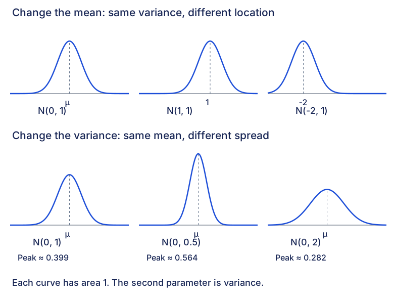
Changing μ shifts location while keeping variance fixed. The source uses $N(0,1)$, $N(1,1)$ and $N(-2,1)$. Changing variance changes spread: at mean 0, compare variances 1,0.5 and 2. Smaller variance gives a narrower, taller curve. The source’s last two spread plots have heights consistent with treating 0.5 and 2 as standard deviations; the accompanying figure here uses them as variances, as the printed notation requires.

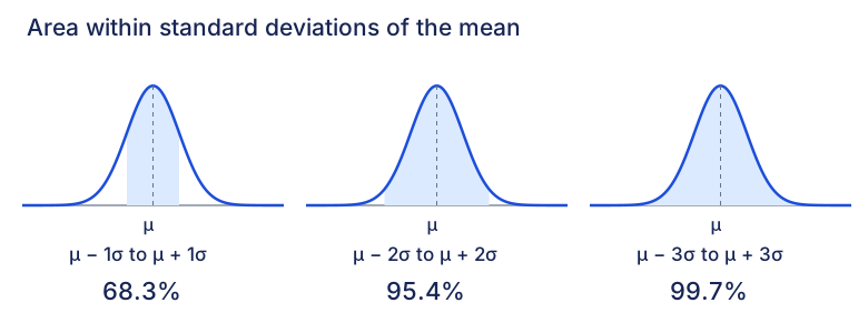
For a normal distribution, approximately 68.3%, 95.4% and 99.7% lie within respectively one, two and three standard deviations of μ. These are central areas, not density heights.

From the shaded area to the calculator

First simplify the inequality, then sketch its region and choose the calculator limits. The source uses normalcdf(lower, upper, μ, σ) to evaluate the density integral. Enter the standard deviation, not the variance. For the examples here, the source uses $-10^{99}$ or $10^{99}$ to simulate an infinite tail to the required precision; those finite numbers are not mathematical infinity.

Example 1 compares interval, right-tail, left-tail and modulus events. Then try all three parts of Self-Practice 1 before opening the working.

Find a cutoff from a probability

The next examples reverse the calculation: the area is given, and the unknown is a boundary. Start with a rough sketch, decide which area is given, and use the standard deviation in invNorm.

For $X\sim N(\mu,\sigma^2)$:

• invNorm(p,μ,σ,LEFT) returns x with $P(X<x)=p$.
• invNorm(p,μ,σ,RIGHT) returns x with $P(X>x)=p$. A left-area-only command uses $1-p$ instead.
• invNorm(p,μ,σ,CENTER) returns two bounds $\mu-a$ and $\mu+a$ such that $P(-a<X-\mu<a)=p$. The bounds must be symmetric about the mean. Each tail has area $(1-p)/2$.

The retained calculator walkthrough uses the tail selector in its stated OS 5.2.2 interface, with STAT WIZARDS ON. If that selector is unavailable, use the equivalent left cumulative area; the probability model does not depend on the interface.

Example 2 contrasts left and right areas, followed by Self-Practice 2. Example 3 uses a central 80% area and both returned endpoints. Pause and think shows why a fixed lower endpoint may require a different route.

Solve a probability inequality using its boundary

The source’s distinction example asks for less than5%, so finding a quantile is only the first step. Find k satisfying the matching equality, then compare the proposed cutoff x with k on a sketch.

For $0<p<1$, a normal lower cumulative area increases as its cutoff moves right; an upper-tail area decreases. The four strict forms are:

Given condition	Boundary used	Required side
$P(X<x)<p$	$P(X<k)=p$	$x<k$
$P(X<x)>p$	$P(X<k)=p$	$x>k$
$P(X>x)<p$	$P(X>k)=p$	$x>k$
$P(X>x)>p$	$P(X>k)=p$	$x<k$

Example 4 keeps the strict real-valued range and then identifies the smallest permissible one-decimal cutoff. The separate self-directed Example 4 retains the source’s repeated number.

Standard normal scores

A standard normal random variable has mean 0 and variance 1: $Z\sim N(0,1)$. It is also called a standard score or z-score. Its density is

$\phi(z)=\frac 1{\sqrt{2\pi}}e^{-z^2/2},\qquad -\infty<z<\infty.$

Standardisation expresses a value in standard deviations from its mean. It lets you compare relative standing in distributions with different spreads and helps solve for unknown μ and/or σ.

The notes ask whether scoring 60% in one test and 65% in another establishes better performance relative to peers.

Raw percentages alone do not: you need the tests’ means and standard deviations. The later source comparison develops this question; no missing data are invented here.

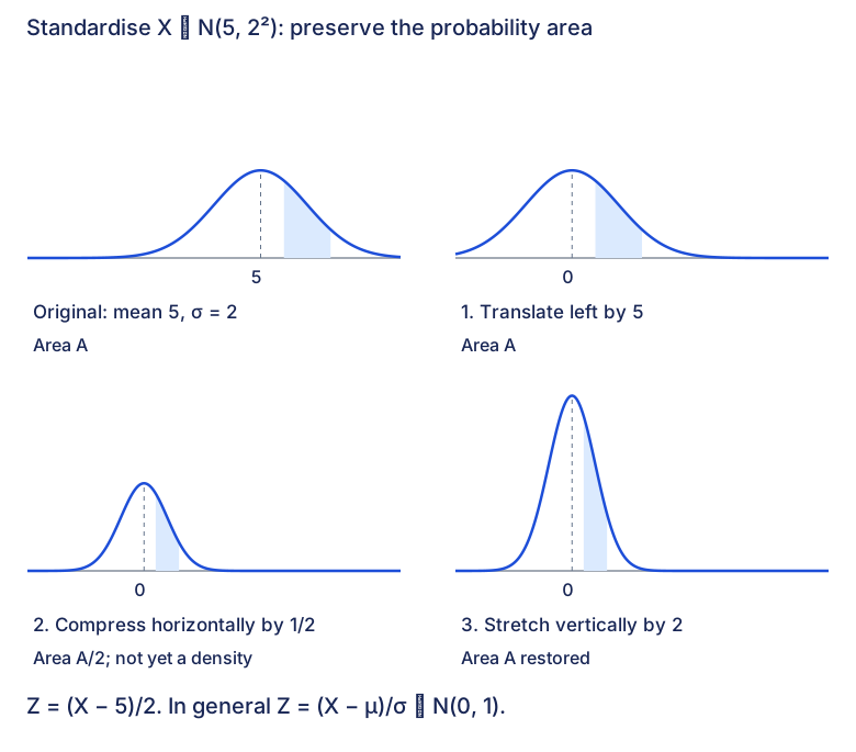
Derive the transformation: first X∼N(5,2²)

The original density is

$g(x)=\frac 1{2\sqrt{2\pi}}e^{-(x-5)^2/8}.$

1. Translate five units left. Replace x with x+5:

$g(x+5)=\frac 1{2\sqrt{2\pi}}e^{-(x+5-5)^2/8}=\frac 1{2\sqrt{2\pi}}e^{-x^2/8}.$

The mean is now 0; the standard deviation remains 2.

2. Compress horizontally by a factor 1/2. Replace x with 2 x in the translated function:

$g(2 x+5)=\frac 1{2\sqrt{2\pi}}e^{-(2 x)^2/8}=\frac 1{2\sqrt{2\pi}}e^{-x^2/2}.$

The width is now that of a standard normal, but the total area has halved. This intermediate curve is not yet a probability density.

3. Stretch vertically by a factor 2. Equivalently replace y with y/2:

$\frac y 2=\frac 1{2\sqrt{2\pi}}e^{-x^2/2}\quad\Longrightarrow\quad y=\frac 1{\sqrt{2\pi}}e^{-x^2/2}.$

The area returns to 1, giving the standard normal density. The corresponding random variable is $Z=(X-5)/2$.

Generalise the three graph transformations

For the normal density $f_X(x)$ with mean μ and standard deviation $\sigma>0$, use the same sequence:

1. Translate parallel to the x-axis by −μ, replacing x with x+μ:

$f_X(x+\mu)=\frac 1{\sigma\sqrt{2\pi}}e^{-(x+\mu-\mu)^2/(2\sigma^2)}=\frac 1{\sigma\sqrt{2\pi}}e^{-x^2/(2\sigma^2)}.$

2. Scale parallel to the x-axis by 1/σ, replacing x with σx in the translated expression:

$f_X(\sigma x+\mu)=\frac 1{\sigma\sqrt{2\pi}}e^{-(\sigma x)^2/(2\sigma^2)}=\frac 1{\sigma\sqrt{2\pi}}e^{-x^2/2}.$

3. Scale parallel to the y-axis by σ, replacing y with y/σ:

$\frac y\sigma=\frac 1{\sigma\sqrt{2\pi}}e^{-x^2/2}\quad\Longrightarrow\quad y=\frac 1{\sqrt{2\pi}}e^{-x^2/2}.$

The source’s graphical argument begins with an interval $x_1<X<x_2$ of area A. Translation leaves area A, with bounds $x_1-\mu$ and $x_2-\mu$. Horizontal scaling gives bounds $(x_1-\mu)/\sigma$ and $(x_2-\mu)/\sigma$ but area A/σ. Vertical scaling multiplies that area by σ, restoring A. Thus

$P(x_1<X<x_2)=P\!\left(\frac{x_1-\mu}{\sigma}<\frac{X-\mu}{\sigma}<\frac{x_2-\mu}{\sigma}\right).$

Both the horizontal and vertical scalings matter for a density graph. For the random variable, standardisation is simply $Z=(X-\mu)/\sigma\sim N(0,1)$; it does not involve another random vertical variable.

Try Self-Practice 3, including the two-tail modulus event.

Confirm standardisation by integration

Define $Z=(X-\mu)/\sigma$, with $\sigma>0$. The source next confirms the preserved area by substitution. Put $z=(x-\mu)/\sigma$, so $dz/dx=1/\sigma$ and $dx/dz=\sigma$. The new limits are $z_1=(x_1-\mu)/\sigma$ and $z_2=(x_2-\mu)/\sigma$.

$P(x_1<X<x_2)=\int_{x_1}^{x_2}\frac 1{\sigma\sqrt{2\pi}}e^{-(x-\mu)^2/(2\sigma^2)}\,dx=\frac 1\sigma\int_{x_1}^{x_2}\frac 1{\sqrt{2\pi}}e^{-\frac 12((x-\mu)/\sigma)^2}\,dx.$

$=\frac 1\sigma\int_{z_1}^{z_2}\frac 1{\sqrt{2\pi}}e^{-z^2/2}\frac{dx}{dz}\,dz=\frac 1\sigma\int_{z_1}^{z_2}\frac 1{\sqrt{2\pi}}e^{-z^2/2}\sigma\,dz.$

$=\int_{z_1}^{z_2}\frac 1{\sqrt{2\pi}}e^{-z^2/2}\,dz=P\!\left(\frac{x_1-\mu}{\sigma}<Z<\frac{x_2-\mu}{\sigma}\right).$

Subtracting μ and dividing by positive σ also gives the same event directly:

$\{x_1<X<x_2\}=\{x_1-\mu<X-\mu<x_2-\mu\}=\left\{\frac{x_1-\mu}{\sigma}<\frac{X-\mu}{\sigma}<\frac{x_2-\mu}{\sigma}\right\}.$

The factor σ from the change in integration width cancels the density’s 1/σ factor. This is the algebraic counterpart of the earlier horizontal and vertical graph scalings. The definition of Z and this calculation establish its standard normal distribution; equality of probabilities alone is not being used to identify two arbitrary random variables on the same sample space.

Use quantiles to find unknown parameters

When μ and/or σ are unknown, the source standardises to $N(0,1)$ before using the given tail probabilities. Example 5 gives one equation for an unknown mean; Example 6 gives two equations for μ and σ. Keep at least 5 significant figures in intermediate working and inspect the meaning of any rounded interval endpoints.

The test-score illustration returns to the earlier 60% versus 65% question with actual means and variances supplied by the source.

Transform one normal variable

For $X\sim N(\mu,\sigma^2)$ and a≠0,

$aX\pm b\sim N(a\mu\pm b,a^2\sigma^2).$

Translation changes the mean but leaves variance unchanged. Multiplication by a changes variance by $a^2$; the standard deviation becomes $|a|\sigma$. The source states the rule for any real a; when a=0, the result is a constant with variance 0, rather than a non-degenerate normal variable.

For the source’s proof, take $Y=aX+b$ with a>0. Its cumulative probability is

$P(Y<y_1)=P(aX+b<y_1)=P\!\left(X<\frac{y_1-b}{a}\right)=\int_{-\infty}^{(y_1-b)/a}\frac 1{\sigma\sqrt{2\pi}}e^{-(x-\mu)^2/(2\sigma^2)}\,dx.$

Set $y=ax+b$, so $dy/dx=a$, $x=(y-b)/a$ and $dx/dy=1/a$. As $x\to-\infty$, $y\to-\infty$; at $x=(y_1-b)/a$, $y=y_1$. Then

$P(Y<y_1)=\int_{-\infty}^{y_1}\frac 1{\sigma\sqrt{2\pi}}e^{-((y-b)/a-\mu)^2/(2\sigma^2)}\frac 1 a\,dy.$

$=\int_{-\infty}^{y_1}\frac 1{a\sigma\sqrt{2\pi}}e^{-(y-a\mu-b)^2/(2 a^2\sigma^2)}\,dy=\int_{-\infty}^{y_1}\frac 1{a\sigma\sqrt{2\pi}}e^{-[y-(a\mu+b)]^2/[2(a\sigma)^2]}\,dy.$

This is the cumulative distribution of $N(a\mu+b,a^2\sigma^2)$. For a<0, dividing the event inequality by a reverses its direction: $P(Y<y_1)=P(X>(y_1-b)/a)$. Accounting for reversed limits gives the density with positive scale $|a|\sigma$ and the same variance $a^2\sigma^2$. The source calls these expressions “cumulative density”; they are cumulative distribution probabilities.

Combine independent normal variables

If X and Y are independent normal variables with respective means $\mu_X,\mu_Y$ and variances $\sigma_X^2,\sigma_Y^2$, then

$aX\pm bY\sim N(a\mu_X\pm b\mu_Y,\ a^2\sigma_X^2+b^2\sigma_Y^2),$

provided the resulting variance is positive. If both coefficients are zero, the combination is a constant. Subtraction changes the mean’s sign but adds the independent variances.

For independent observations $X_1,\ldots,X_n$, each $N(\mu,\sigma^2)$,

$X_1+\cdots+X_n\sim N(n\mu,n\sigma^2),\qquad n\ge 1.$

The complete source expectation/variance summary is:

Property	Expectation	Variance
Constant a	$E(a)=a$	$\operatorname{Var}(a)=0$
Scale one variable	$E(aX)=aE(X)$	$\operatorname{Var}(aX)=a^2\operatorname{Var}(X)$
Scale and translate	$E(aX\pm b)=aE(X)\pm b$	$\operatorname{Var}(aX\pm b)=a^2\operatorname{Var}(X)$
Combine two variables	$E(aX\pm bY)=aE(X)\pm bE(Y)$; independence is not required	For independent X,Y: $\operatorname{Var}(aX\pm bY)=a^2\operatorname{Var}(X)+b^2\operatorname{Var}(Y)$

The source warns against applying the variance sum without independence. More precisely, independence is sufficient, and without it the omitted covariance term may matter:

$\operatorname{Var}(aX\pm bY)=a^2\operatorname{Var}(X)+b^2\operatorname{Var}(Y)\pm 2 ab\operatorname{Cov}(X,Y).$

Zero covariance can also make the variance sum valid; it alone does not establish that an arbitrary combination of marginally normal variables is normal. The independent-normal rule above supplies both the distribution and its variance.

One scaled observation or several observations?

The notes distinguish nX, n times one observation of one object, from $X_1+\cdots+X_n$, the sum of n independent observations from n objects. For n>1 and positive σ², their variances differ:

$nX\sim N(n\mu,n^2\sigma^2),\qquad X_1+\cdots+X_n\sim N(n\mu,n\sigma^2).$

Words like “twice” or “thrice” usually mean scaling; “sum of” usually combines observations. Always inspect the actual objects and independence assumptions. The source’s translation reminder also follows from the table: shifting every value by the same constant changes the mean and leaves the variance unchanged.

Self-directed learning: normal approximation to a binomial

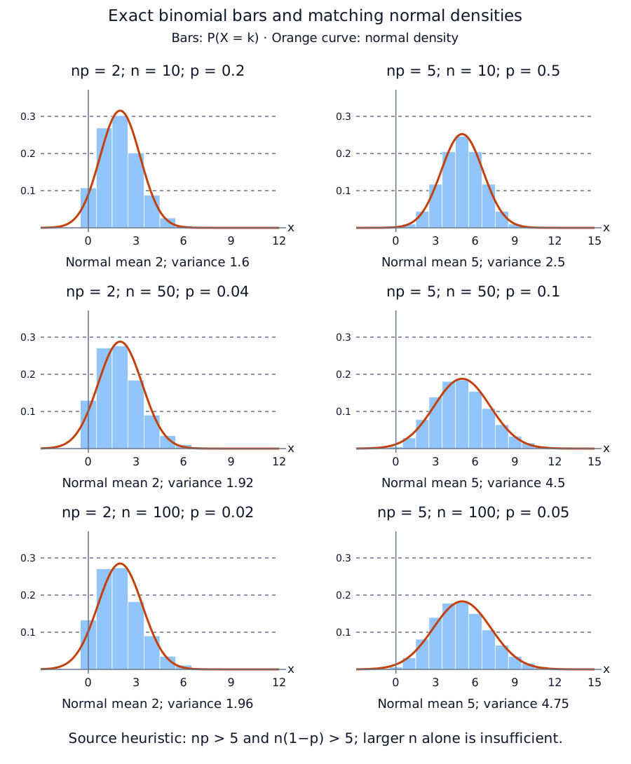
For $X\sim B(n,p)$ the source compares binomial probability bars with a matching normal curve, keeping $np$ constant while increasing $n$. Its six panels use $np=2$ or $np=5$, each with $n=10,50,100$. The reconstruction below calculates $p=(np)/n$ and overlays the density of $Y\sim N(np,np(1-p))$. Binomial bar heights are point probabilities; a normal density height is not itself a point probability.

The source’s general rule is $np>5$ and $n(1-p)>5$. Keep the strict inequalities as printed. This is a practical approximation heuristic, not a universal accuracy guarantee, particularly for far tails. Increasing $n$ while holding a small $np$ fixed does not force a good normal approximation: the $np=2$ panels remain skewed. The $np=5$ panels are at the stated threshold, rather than satisfying $np>5$.

Independently authored use note: for a count event, continuity correction aligns an integer bin with a continuous interval; for example, $P(X\le k)\approx P(Y<k+1/2)$. Check the actual event and approximation quality rather than substituting a normal density value for a probability. Exact binomial probabilities remain available.

The printed optional resources are GeoGebra simulation and fixed-np exploration. These are retained source pointers; their remote contents have not been reviewed here.