Sampling and the sample mean
Choose a sampling model, estimate population parameters and distinguish exact normal results from CLT approximations.
← Back to learning units · Complete chapter reading and print view · Open reference notes separately
By the end, you can
- Separate a population parameter from a sample statistic
- Find the mean and standard error of a sample mean
- Use unbiased variance estimation and the CLT with care
about 35 minutes for the lesson · practise at your own pace.
The central idea
Population parameters are fixed; sample statistics vary across repeated samples. For iid observations with mean and finite variance , and . An exact normal population gives an exact normal mean; otherwise a suitable large-sample CLT approximation may apply. Use in the unbiased variance estimate, and keep sampling bias separate from sampling variability.
Compare all five sampling distributions
Expand diagramFit diagram to page
Use the scrollbars or arrow keys to inspect details.
Explore
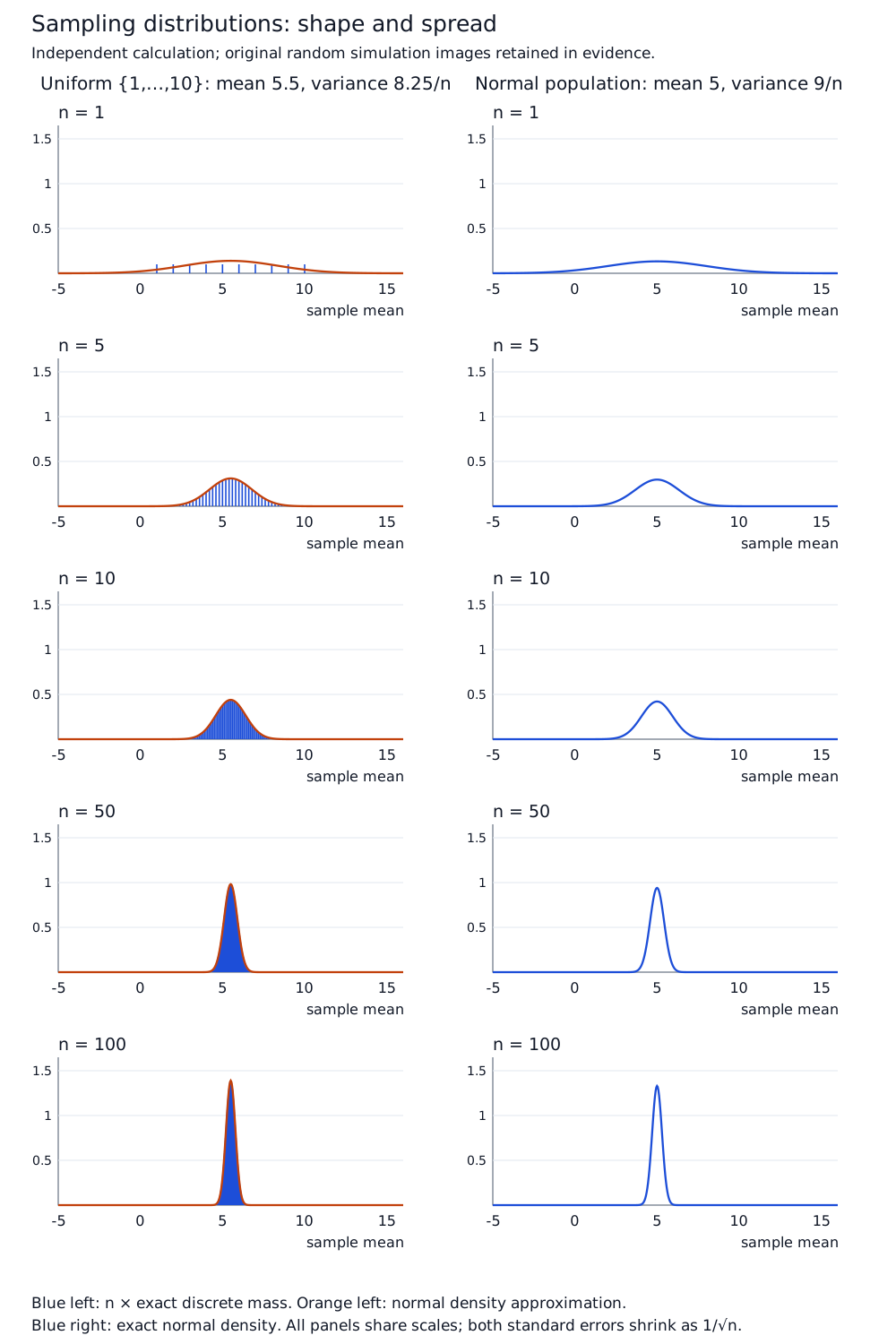
The source compares independent samples from uniform on and for .
| x | 1 | 2 | 3 | 4 | 5 | 6 | 7 | 8 | 9 | 10 |
|---|---|---|---|---|---|---|---|---|---|---|
| 0.1 | 0.1 | 0.1 | 0.1 | 0.1 | 0.1 | 0.1 | 0.1 | 0.1 | 0.1 |
Here , , so the mean has variance . The distribution is flat rather than normal; as grows, the exact discrete mean distribution becomes bell shaped and concentrates near 5.5. For , the mean is exactly for every listed . Both spreads shrink like .
| n | ||
|---|---|---|
| 1 | 8.25 | 9 |
| 5 | 1.65 | 1.8 |
| 10 | 0.825 | 0.9 |
| 50 | 0.165 | 0.18 |
| 100 | 0.0825 | 0.09 |
The figure is an independent mathematical reconstruction: exact discrete convolutions are shown for and exact normal densities for , with a normal approximation overlaid for comparison.
It does not recreate the source’s random simulation run. Its ten original simulation chart images remain in the review evidence.
For a spreadsheet experiment, generate many independent size- samples, calculate each mean, and plot the means while keeping the population distribution fixed. Compare the observed centre and variance with the table.
The lecture links two external simulations: uniform discrete population and normal population. These are preserved source references; their external contents have not been reviewed. The Example 10 enrichment QR decodes to estimation theory; unbiased estimation is one form of estimation, and the destination is also outside this source review.
Before viewing each comparison, predict the centre, variance and shape of the distribution of means. In a spreadsheet, keep a separate plot of the individual observations. Explain why increasing the number of repeated samples makes the plot more stable, while increasing the size of each sample changes the spread of the means.
Worked example
Independent component measurements are normally distributed with population mean 100 and known standard deviation 6. Let be one measurement and let be the mean of nine independent measurements. Then , while exactly.
For a mean above 104, the standardised boundary is , giving .
For one measurement above 104, it is , giving .
Sketch both curves around the same centre: the mean has the smaller spread. No CLT approximation is needed because the population is normal.
The standard deviation of a mean is $\sigma/\sqrt n$, not $\sigma/n$. More observations reduce the variability of the mean; they do not change the distribution of a single measurement.
Check your understanding
Five independent randomly selected observations from a population of unspecified shape give and . Estimate the population mean and variance. Can these summaries justify calculating an exact normal probability for the sample mean? If the same sampling process is used with 20 observations, what happens to the theoretical standard error, and would that repair a biased sampling frame?
The mean estimate is . The unbiased variance estimate is .
These estimates do not determine the population shape or make a size-five mean exactly normal; a justified population model or approximation is still needed.
For the same population under independent sampling, the theoretical standard error changes from to , so it halves.
A larger sample does not repair a biased frame. The calculated is an estimate of spread, not a known population standard deviation.
Mastery learning objectives
At the end of this chapter, I should be able to:
Choose a practice question
| Common question type | Lecture examples | Discussion | Review follow-up |
|---|---|---|---|
| Unbiased estimates using calculator | 2, 3 | 1 | 1 |
| Unbiased estimates using summarized data | 2, 3, 4, 10 first part | 2 | 2 |
| Means from normal populations | 5, 6 | 3(b), 4(iv), 5(b)(i), 6 | 7, 10 |
| CLT for means | 7, 8, 9, 10 | 5(a),(b)(ii)(iii), 7 | 3, 4(ii), 6(vi), 5(b), 7(a), 9(iii), 10(iv) |
| Prior topic: discrete random variables | — | — | 9(i)(ii) |
| Prior topic: binomial distribution | — | 4(ii) | 4(i), 5(a) |
| Prior topic: normal distribution | — | 3(a), 4(i)–(iii) | 5(b), 6(i)–(v), 8(ii), 10 |
The printed CLT row labels Example 10 “1st part”; its first part estimates parameters and the later probability part uses CLT. The map preserves the reference and explains its intended skill. The printed map also places Review 5(b) in normal prerequisites although its binomial daily count needs a CLT approximation; follow the model explained in that question.
Both lecture copies repeat all seven Discussion questions on PDF25–26 and all ten Review questions on PDF27–30. These links point to the already source-compared questions, preserving separate source occurrences through aliases.
Discussion short answers agree with the retained solutions.
The Review short key mislabels 5(b) as (c), 6(vi) as (iv), and 8(ii)(a)/(b) as (b)(i)/(ii); it labels 10(ii) .0882 as(i) and 10(iii) .375 as(ii), and omits 10(i)’s roots.
Canonical working retains the actual asks and the complete answer. Native keys stay unchanged. No marks are printed for the lecture examples or Discussion; the repeated Review retains 75 marks in its canonical records.
Practice questions
Practice section 1 · Questions 1–6
Select thirty distinct students fairly · Estimate mean and variance from seven raw values · +4 more
Practice section 2 · Questions 7–12
Separate a binomial mean approximation from its exact total · Approximate mean daily wine production · +4 more
- Separate a binomial mean approximation from its exact total
- Approximate mean daily wine production
- Compare two independent sample means
- Estimate a population, then qualify a plug-in tail probability
- Estimate population mean and variance from a frequency table
- Use raw and shifted summaries for unbiased estimates
Practice section 3 · Questions 13–18
Separate individual observations from a normal sample mean · Combine normal observations and choose a minimum sample size · +4 more
- Separate individual observations from a normal sample mean
- Combine normal observations and choose a minimum sample size
- Distinguish CLT estimates from exact probabilities and strict thresholds
- Choose a sample size from an exact normal mean distribution
- Translate between a sample mean and a total
- Estimate emissions mean and variance from test data
Practice section 4 · Questions 19–24
Define a random sample and use shifted totals · Approximate a binomial sample mean and track its endpoints · +4 more
- Define a random sample and use shifted totals
- Approximate a binomial sample mean and track its endpoints
- Distinguish a binomial tail from a CLT mean tail
- Find a binomial game limit and a daily-average probability
- Align clock times before comparing normal travel times
- Infer a normal standard deviation from symmetric tail areas
Practice section 5 · Questions 25–27
Recover normal parameters and combine independent masses · Find a repeat-draw distribution and approximate its sample mean · +1 more
Ready to try this on your own?
For “Sampling and the sample mean”, try a question without the working and explain your method. This records your confidence, saved in this browser only.