Worked solution
Calculate correlation and investigate a radiation outlier
The data show the intensity of radiation from a substance after time .
| 0.2 | 3 |
| 0.4 | 3.5 |
| 0.6 | 1.3 |
| 0.8 | 0.6 |
| 1.0 | 0.4 |
| 1.2 | 0.2 |
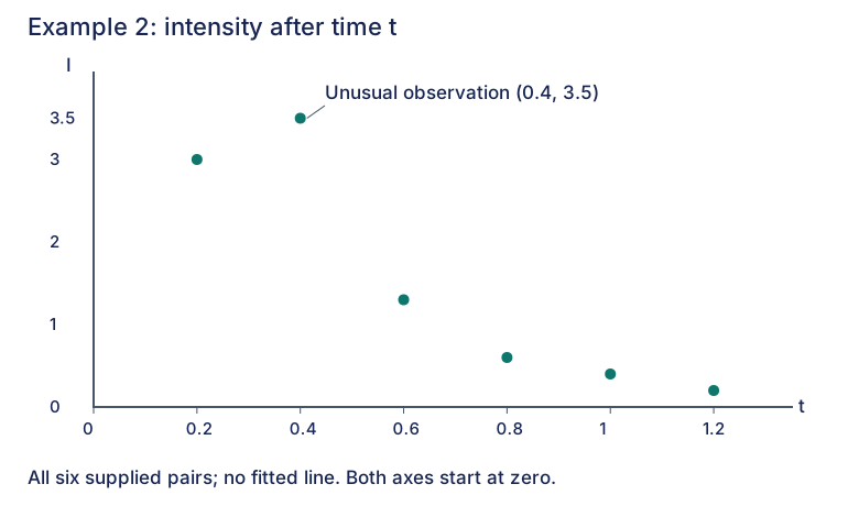
(i) Use a suitable diagram to explain why the product moment correlation coefficient between and is negative and not very close to .
(ii) By using the formula for , calculate the product moment correlation coefficient between and .
(iii) State the coordinates of a point in the diagram in (i) which does not seem to follow the linear trend. If it is removed, without any calculations, explain why is closer to .
CJC · Lecture · Example 2
(i) Explain the sign and imperfect fit
Answer
The overall scatter falls as increases, but the points do not all lie close to one falling line.
Plot horizontally and vertically, keeping all six pairs. In particular, sits above the main falling trend. The source directs you to the six-step plotting procedure in Example 1 and identifies time as explanatory and intensity as response. The first pair is , not . The source plot shows the endpoints 0.2 and 1.2 on the time axis and intensity extrema 0.2 and 3.5. This reconstruction labels a true zero origin. The sign follows the overall downward association; the visible blank explanatory answer is completed here from the supplied data.
(ii) Obtain the paired-data totals
Answer
, , , , , .
Keep in L1 and in L2. Press STAT, choose CALC, then 2:2-Var Stats. Enter L1 as Xlist with 2nd 1, and L2 as Ylist with 2nd 2. Highlight Calculate, then ENTER; scroll up/down for all totals. Map calculator to and to . The source screenshots also show , , , and . The correlation formula uses the displayed sums, not a mixture of sample and population standard deviations.
(ii) Substitute into the printed formula
Answer
(3 s.f.).
Use the required formula rather than only reporting a calculator correlation:
The printed worked value is to 3 significant figures. The source notes that a direct calculator method for will be illustrated in later regression examples; that does not replace the formula requested here.
(iii) Reason about removal without recalculating
Answer
Remove . The remaining points lie closer to a falling straight line, so is closer to .
The remaining scatter still falls as time increases but is less dispersed around a negative linear trend. This is the graphical explanation requested; a new numerical coefficient is unnecessary. The visible Student answer on PDF page 12 is blank, so this is an authored completion checked against the six exact pairs, not a supplied Teacher answer.
Compare your sketch
Expand diagramFit diagram to page
Use the scrollbars or arrow keys to inspect details.
Common mistakes
Keep the unusual observation when calculating part (ii). Part (iii) asks for a graphical explanation without recalculating.
Solution notes
Only a Student lecture PDF is supplied. The formula substitution and calculator procedure are printed; the blank explanations in (i) and (iii) are completed explicitly from the data. No marks are printed.