Find the mean and variance of defective-part counts

$E(X)=0(0.51)+1(0.38)+2(0.10)+3(0.01)=0.61$. Thus $\mu=0.61$.

Use $\operatorname{Var}(X)=E[(X-\mu)^2]=\sum_x(x-\mu)^2f(x)$. The complete source table is

$\operatorname{Var}(X)=0.51(0.3721)+0.38(0.1521)+0.1(1.9321)+0.01(5.7121)=0.4979$.

Use $\operatorname{Var}(X)=E(X^2)-[E(X)]^2$. From the same four probabilities, $E(X^2)=0^2(0.51)+1^2(0.38)+2^2(0.10)+3^2(0.01)=0.87$. Hence $\operatorname{Var}(X)=0.87-0.61^2=0.4979$.

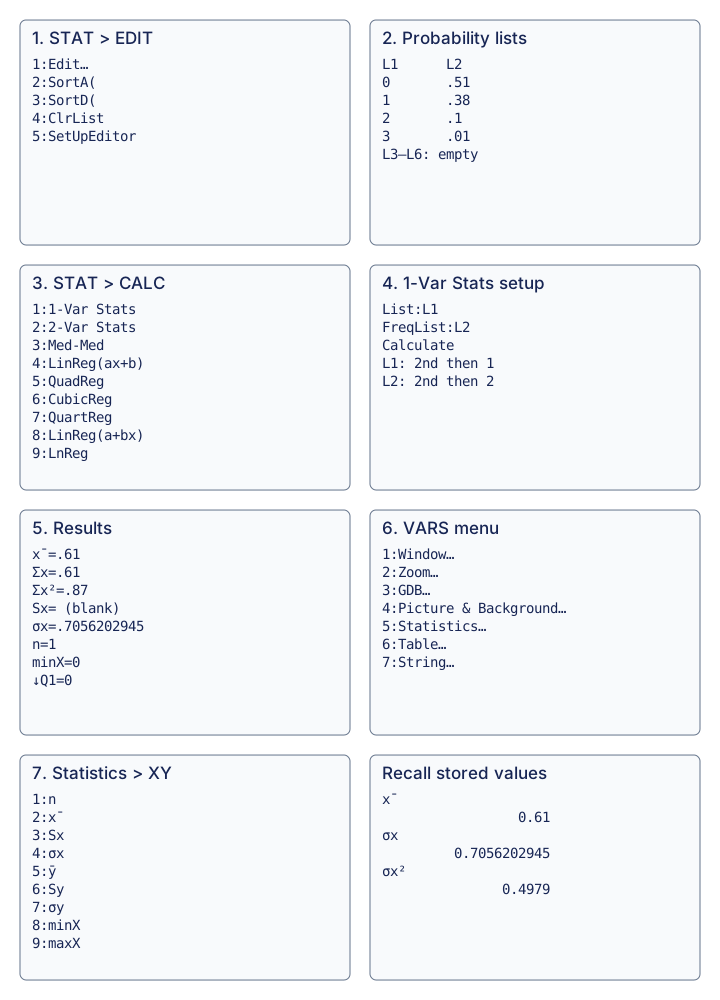
Use the graphing calculator as the source’s third method for Example 11:

1. Press STAT, then 1:Edit, to enter the distribution.
2. Put $0,1,2,3$ in L1, and the corresponding probabilities $0.51,0.38,0.10,0.01$ in L2.
3. Press STAT, choose CALC, then 1:1-Var Stats.
4. Set List:L1 and FreqList:L2. Obtain L1 with 2nd, 1 and L2 with 2nd, 2.
5. Highlight Calculate and press ENTER. The printed screen shows $\bar x=0.61$, $\Sigma x=0.61$, $\Sigma x^2=0.87$, $\sigma_x=0.7056202945$, $n=1$, minX=0 and Q1=0; Sx is blank. Scroll down for more statistics.
6. To avoid retyping a rounded value, press VARS, then 5:Statistics.
7. Choose 2: x̄ for the mean or 4: σx for the population standard deviation. Recall the stored $\sigma_x$ and square it: the displayed $\sigma_x^2=0.4979$ is the variance. The source explains that this workflow supplies standard deviation rather than variance directly.

Use σx, not Sx. Here the frequency weights are probabilities and sum to one, so the printed n=1 is the total weight, not one observed defective part. The source’s squared stored value avoids premature rounding. The diagram retains the meaningful source menu and screen contents.