Worked solution
Compare pollution models and audit a damaged regression fragment
(a) Traffic engineers compare traffic flow on a busy main road with air pollution at a nearby monitoring station. Each hour, sensors report the average traffic flow (vehicles per hour) for the preceding hour; the station supplies a pollution reading in a suitable unit, with higher readings indicating more pollution. A random sample of eight hours gives:
| 1796 | 1.0 |
| 1918 | 2.2 |
| 2120 | 3.5 |
| 2315 | 4.2 |
| 2368 | 4.3 |
| 2420 | 4.5 |
| 2588 | 4.9 |
| 2850 | 5.5 |
(i) Draw the scatter diagram, labelling the axes.
Two proposed models are and .
(ii) Find the correlation coefficient between (a) and , and (b) and .
(iii) Use (i) and (ii) to explain which model is better.
(iv) Find a suitable regression equation and use it to estimate when .
(v) Comment on the validity of the headline “Heavy traffic causes air pollution” in light of these results.
(b) A partly destroyed research paper retains these statements: the mean of is 4.4; the regression of on is ; the regression of on begins . Calculate the missing constant at the end of the second equation.
[2017/JJC/II/10]
CJC · Discussion · Question 6
(a)(i) Preserve the hourly paired observations
Answer
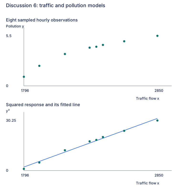
The eight observations rise with decreasing apparent slope.
Plot average traffic flow horizontally and the corresponding hourly pollution reading vertically. The original response shows a curved increasing pattern; the independently drawn second panel shows the squared-response transformation considered below. The sampling unit is an hour, not eight different stations or eight vehicles.
(a)(ii)(a) Correlate the original variables
Answer
(3 s.f.).
Using all eight pairs gives , matching the printed . Despite the large positive value, inspect the curved scatter before selecting a straight response model.
(a)(ii)(b) Correlate flow with squared pollution
Answer
(3 s.f.).
Square each pollution reading while retaining its matching traffic flow. The coefficient is , matching the printed . This transformation is of the response, not of flow.
(a)(iii) Compare the two proposed forms
Answer
is the better of these two sample models.
The original scatter curves and flattens, while the squared-response scatter is close to a straight rising line and has a correlation closer to 1. Together these support the transformed candidate. This compares fit to this sample; it does not establish a causal mechanism or a universally valid law.
(a)(iv) Fit squared pollution on flow
Answer
Predicted reading (2 s.f.).
The full independently calculated regression is , with
matching the printed rounded form . With the unrounded coefficients,
Take the positive root, consistent with the supplied positive pollution scale and observations. 2000 vehicles per hour is within 1796–2850; this is interpolation. The source prints 2.8 without a precision instruction, so that displayed result is preserved; 2 s.f. states its precision rather than inventing a printed requirement.
(a)(v) Evaluate the headline
Answer
The results show association; they do not by themselves establish the causal headline.
The sampled hourly observations do not control possible factors such as weather or other pollution sources. Those are possible unmeasured influences, not data supplied by the question. A transformed coefficient close to 1 does not establish that changing traffic alone causes the observed pollution change.
(b) Compute the formal constant and check consistency
Answer
The missing number is , giving formally ; the supplied slopes are inconsistent.
Both genuine regression lines pass through the mean point. From the first equation,
Write the fragment as ; then
which reproduces the printed missing-number answer. However, for a nondegenerate paired dataset, the product of the two regression slopes equals . Here , so these cannot both be the least-squares regressions of the same data. The formal mean-point completion is retained, but the source fragment is mathematically inconsistent as stated. No corrected slope or replacement dataset is invented.
Compare your sketch
Expand diagramFit diagram to page
Use the scrollbars or arrow keys to inspect details.