Worked solution
Compare used-car prices with reciprocal mileage
Adriana investigates how used-car prices depend on distance driven. A UK website lists seven cars of the same make and model; distance is in miles and price is in pounds sterling.
| (miles) | (pounds sterling) |
|---|---|
| 14588 | 12450 |
| 8954 | 15200 |
| 24030 | 11900 |
| 37551 | 10700 |
| 45452 | 10600 |
| 30100 | 10900 |
| 5055 | 22500 |
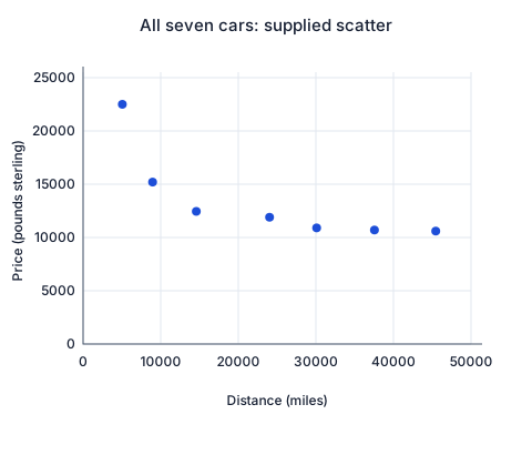
The source supplies the scatter diagram shown here and the correlation coefficient .
(a) What conclusion should Adriana reach about the relationship between and ? Justify your answer.
(b) Would the coefficient differ if distances were converted to kilometres and prices to Singapore dollars? Use the given conversions: 1 mile = 1.6 kilometres; 1 pound sterling = 1.7 Singapore dollars.
Adriana discovers that the car with and is a special version with a bigger engine and many extra features.
(c) Explain why this special car should not be used in the analysis.
For the rest of the question, exclude this special car.
(d) Use a reciprocal transformation to sketch against . Draw a line of best fit by eye.
(e) Mark the distances used to obtain the least-squares regression of on . Explain why these distances are squared and why the method is called least squares.
(f) Use your calculator to find this least-squares regression equation and the corresponding correlation coefficient.
(g) Estimate the price of an ordinary car of this make and model that has travelled 5055 miles. Explain whether the estimate is likely to be reliable.
Expand diagramFit diagram to page
Use the scrollbars or arrow keys to inspect details.
CJC · Discussion · Question 8
(a) Read the scatter together with the coefficient
Answer
Price tends to decrease as mileage increases; the scatter is curved.
The supplied indicates fairly strong negative linear association, but the seven plotted observations show a decreasing curve that levels off. Thus a decreasing relationship is supported; a coefficient of this size alone does not make a straight-line price model appropriate.
(b) Rescale both variables positively
Answer
The coefficient remains .
The new variables are and . Multiplying each variable by a positive constant changes the units without changing correlation. These are the conversion rates supplied for this exercise.
(c) Keep the comparison population consistent
Answer
Exclude the special version from the ordinary-model analysis.
Its larger engine and extra features affect price in addition to mileage. The remaining cars are intended to represent the ordinary version, so treating this distinct specification as comparable would mix populations. The exclusion is supported by the supplied specification information, rather than merely by an inconvenient position on the scatter. Use only the first six pairs in (d)–(g).
(d) Transform the six comparable cars
Answer
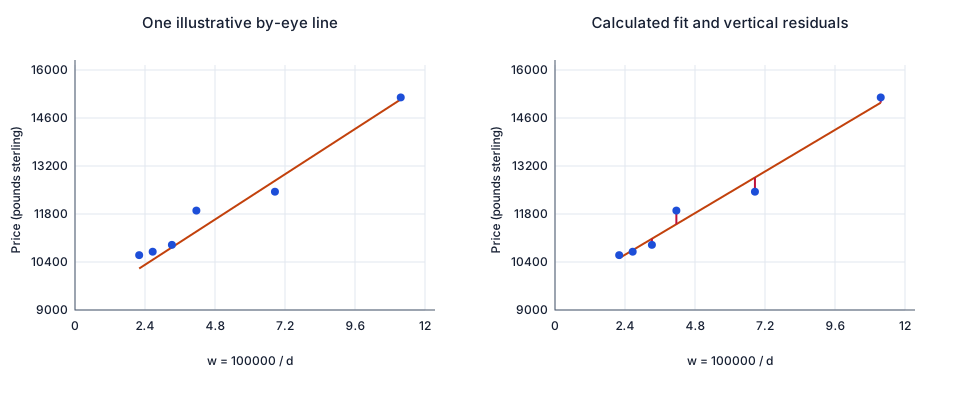
Plot horizontally and vertically; the six points are close to a rising line.
Retain the pairings and use the unrounded transformed values for fitting:
| (shown to 4 d.p.) | ||
|---|---|---|
| 14588 | 6.8549 | 12450 |
| 8954 | 11.1682 | 15200 |
| 24030 | 4.1615 | 11900 |
| 37551 | 2.6630 | 10700 |
| 45452 | 2.2001 | 10600 |
| 30100 | 3.3223 | 10900 |
A sensible by-eye line runs through the middle of the transformed points. The diagram illustrates as one possible hand-drawn choice, not a unique answer or the calculator regression requested in (f).
(e) Mark the response residuals
Answer
Use vertical price residuals and minimize their sum of squares.
For a candidate line , mark the vertical segment at each observed , from the fitted price to the observed price . The signed residual is ; the geometric segment has length . Squaring prevents positive and negative residuals from cancelling and weights larger discrepancies more heavily. Least squares chooses the coefficients minimizing . The second diagram marks these vertical segments for the computed regression; horizontal or perpendicular distances solve different fitting problems.
(f) Fit price on reciprocal mileage
Answer
; (printed rounded results).
Fitting on with the six comparable cars gives , with
The coefficient is , which rounds to the printed 0.987. Rounding the fitted intercept and slope gives , equivalently the printed . The original negative coefficient concerned ; the transformed variable decreases as increases, so the positive transformed coefficient is consistent with decreasing price as mileage increases.
(g) Predict for an ordinary car at 5055 miles
Answer
Estimated price: £19400; reliability is limited by extrapolation.
Using the full coefficients from (f),
which gives the printed £19400 to 3 significant figures. The target mileage 5055 is below the comparable sample range 8954–45452, so this is extrapolation; the transformed input is also beyond the observed reciprocal range. The actual £22500 car at 5055 miles was the special version and remains excluded. It does not provide a comparable observation that validates this prediction for an ordinary car.
Compare your sketch
Expand diagramFit diagram to page
Use the scrollbars or arrow keys to inspect details.
Solution notes
All seven asks, seven original pairs, supplied units/correlation, special-version information and exclusion for (d)–(g) retained. Printed equation, transformed coefficient and prediction preserved. Working, by-eye illustration, exact-data scatter reconstructions and residual diagram authored. No printed marks or exam reference.