Worked solution
Compare fuel-consumption models using squared residuals
Abi and Bhani measure fuel consumption (kilometres per litre) for a car driven at different constant speeds (kilometres per hour).
| 40 | 22 |
| 45 | 20 |
| 50 | 18 |
| 55 | 17 |
| 60 | 16 |
(i) Abi models the data with .
(a) On graph paper, draw a scatter diagram of the data and the line .
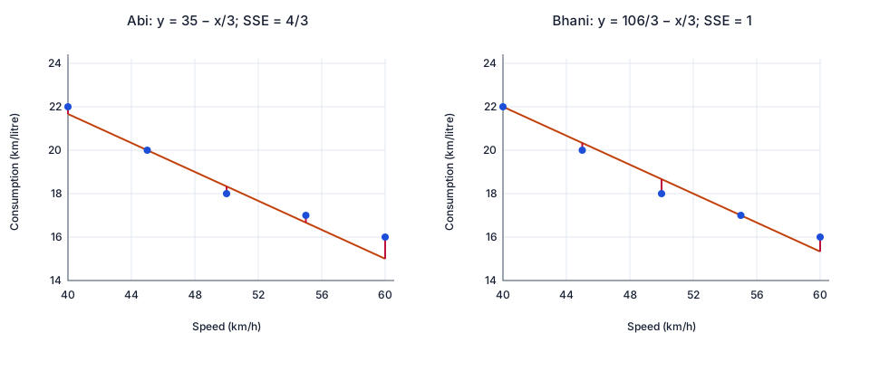
(b) For a fitted line , the source describes the residual at as the vertical distance between and . Mark each residual on the diagram.
(c) Calculate the sum of squared residuals for Abi’s line.
(d) Explain why, in general, the sum of squared residuals is used instead of the sum of residuals.
Bhani uses a line through and . The sum of squared residuals for Bhani’s line is 1.
(ii) State, with a reason, which model gives a better fit.
(iii) Cerie carries out a similar experiment on a different car. Her fitted line has a sum of squared residuals of 0. What can you deduce about her data points?
[N2019/II/10(modified)]
CJC · Discussion · Question 9
(i)(a) Plot all observations and Abi’s proposed line
Answer
Plot the five pairs and .
Use speed (km/h) horizontally and consumption (km/litre) vertically. For example, Abi’s line passes through and . The diagram retains the five measured pairs and a coordinate grid. This is the supplied candidate line, not a newly computed least-squares regression.
(i)(b) Draw the vertical differences
Answer
Signed residuals: .
At each recorded speed, subtract the fitted consumption from the observation:
| 40 | 22 | ||
| 45 | 20 | 20 | 0 |
| 50 | 18 | ||
| 55 | 17 | ||
| 60 | 16 | 15 | 1 |
Mark a vertical segment between each observation and its fitted point. At speed 45 the residual is zero, so its segment has zero length. The source’s geometric distances are the magnitudes of these signed residuals; squaring either gives the same result.
(i)(c) Sum the squared residuals
Answer
.
Using the exact residuals,
This agrees with the printed answer 1.33. Keep the thirds unrounded until the final result.
(i)(d) Prevent cancellation of errors
Answer
Squaring prevents signed errors from cancelling.
Positive and negative residuals can cancel in an ordinary sum even when the observations are far from the line. Squared residuals are all nonnegative and give larger discrepancies greater weight. If the source’s word “distance” is interpreted as unsigned length, such lengths already cannot cancel; the conventional residual here is signed. Minimizing squared residuals is the stated criterion, distinct from minimizing absolute distances.
(ii) Compare the same error criterion
Answer
Bhani’s line fits these observations better: .
Bhani’s slope is and intercept is . Its residuals are , whose squares sum to 1, matching the given value. Since both lines are compared on the same five observations and the same vertical squared-error criterion, Bhani’s smaller total gives the better of these two fits. This comparison does not establish that Bhani’s line is the globally optimal least-squares line.
(iii) Interpret zero error for Cerie’s different car
Answer
Every observed point lies exactly on Cerie’s fitted line.
Each squared residual is nonnegative. Their sum can be zero only if every residual is zero, so each measured point is on her line. The question supplies no Cerie data, slope or intercept: none can be inferred. This exact sample fit does not by itself guarantee the relationship at other speeds or for other cars.
Compare your sketch
Expand diagramFit diagram to page
Use the scrollbars or arrow keys to inspect details.
Solution notes
All six printed asks, both graphing tasks, five observations, Abi equation, Bhani defining points/given SSE 1, Cerie different-car context and printed 1.33 retained. Exact arithmetic and signed-versus-geometric residual qualification authored; no printed marks.