Correlation and linear regression
← Back to learning units · Complete chapter reading and print view · Open reference notes separately
By the end, you can
- Use scatterplots before fitting a line
- Interpret correlation without claiming causation
- Distinguish interpolation, extrapolation and transformed models
about 40 minutes for the lesson · practise at your own pace.
The central idea
Correlation describes linear association, while a regression line predicts a response from an explanatory variable. The least-squares line minimises squared vertical residuals. A strong association does not establish causation. Prediction beyond the observed input range is extrapolation; transformations can reveal a relationship hidden in the original coordinates.
Begin with paired observations
The notes ask about links between GenAI use and examination scores, and between temperature and rainfall intensity. These are questions to investigate, not established conclusions. In the source’s controlled experiment, vary the slope angle through and record a ball’s travel time. The angle is the independent (explanatory) variable, and the travel time is the dependent (response) variable.
When control is impractical, the source proposes observing temperature and sea level each day over ten years. This is observational data collection. The notes use “natural experiments” broadly here; an observational study is not automatically a natural experiment with an externally imposed change. Controlled studies are possible in some settings even in fields mentioned by the source; identify what is actually controlled in the particular investigation.
Bivariate data consist of ordered pairs , such as each person’s age and salary. Each pair must refer to the same observation. The explanatory variable supplies the basis for prediction or study; the response is the outcome observed or predicted. In an observational study the explanatory variable need not be manipulated. Calling a variable “independent” in this role does not assert statistical independence of X and Y.
Try the five source situations before opening their working.
Inspect a scatter diagram
A scatter diagram plots the paired numerical observations, usually with the explanatory variable on the horizontal x-axis and the response on the vertical y-axis. The notes also call it a scatter plot, scatter graph or scatter chart. Inspect:
- Shape: approximately linear, curved (such as the source’s inverted U), or another pattern (such as its loop).
- Direction for a linear pattern: positive/direct means y tends to rise with x; negative/inverse means y tends to fall with x. “Inverse” here describes direction, not a proved reciprocal formula .
- Strength of the linear pattern: tight clustering about a line is stronger than a widely scattered cloud. A strong curved pattern need not have strong linear correlation.
All eight schematic panels from the opening notes are reconstructed in the accompanying figure: three shape examples, two direction examples and three strength examples. They are illustrations, not measured numerical data.
The source uses numerical variables such as height, mass, rates and counts. It contrasts beauty and happiness as not directly numerical. Such concepts can be studied using explicitly defined numerical scores, but a score’s meaning and measurement quality need justification; merely assigning category numbers does not establish a quantitative scale.
For the linear correlation studied here, the source’s sequence is sketch the scatter diagram, then find the correlation coefficient. Plotting first can reveal curvature or unusual observations hidden by a single summary number.
Transfer a calculator plot to a clear sketch
Retain all five source pointers:
- Check the window scale: the origin may not be visible.
- Label both axes and put the explanatory variable horizontally, response vertically.
- Mark the minimum and maximum x and y values.
- Match the number of observations with the number of plotted dots or crosses. Coincident pairs can overlap, so record their multiplicity if needed.
- Preserve relative positions accurately. Graph paper is unnecessary unless requested.
Example 1 retains every data pair and the complete six-step calculator route before describing the observed pattern.
Eight scatter patterns
Read shape, direction and scatter
Compare the patterns below.
Linear relationship
6 points
Curved: inverted U
9 points
Curved: loop
8 points
Positive linear
5 points
Negative linear
5 points
Strong negative linear
4 points
Strong positive linear
6 points
Weak/no clear linear
13 points
- Schematic illustrations: positions are not measured observations. No numerical data or calculated correlation is implied.
- Look for shape before describing direction or strength.
- A clear curved relationship can have little or no linear correlation.
Five coefficient cases
Compare five correlation cases
Compare the patterns below.
Perfect negative · r = −1
3 points
Negative · −1 < r < 0
3 points
Zero linear correlation · r = 0
8 points
Positive · 0 < r < 1
3 points
Perfect positive · r = +1
3 points
- Schematic illustrations: positions are not measured observations. No numerical data or calculated correlation is implied.
- The coefficient labels retain the roles stated in the source, not values computed from these schematic positions.
- Zero linear correlation does not imply independence or no relationship.
Causation and equal-coefficient patterns
Read the scatter as well as the coefficient
Compare the patterns below.
Left and right foot size
5 points
Linear-looking scatter · source r = 0.86
11 points
Curved pattern · source r = 0.86
11 points
One unusual observation · source r = 0.86
11 points
- Ringed point: Unusual observation in this schematic.
- Strong correlation alone does not establish causation. In the foot-size example, shared influences such as genes can explain the association.
- The source reports r = 0.86 for each of the three original data sets below the foot-size illustration. These reconstructed positions are schematic; they are not the raw data used to calculate that coefficient.
- A coefficient alone does not reveal curvature or an unusual observation. Inspect the diagram before interpreting a linear relationship.
Outlier in a rising scatter
Inspect how an outlier changes the pattern
Compare the patterns below.
Source outlier in a rising pattern
14 points
- Ringed point: Source outlier (2, 7).
- The source identifies (2, 7) exactly. Other point positions in this reconstruction are schematic; no complete numerical data set is supplied.
- In this example, the source states that removing (2, 7) raises the positive correlation because the remaining pattern is closer to a rising straight line.
- An outlier can increase or decrease a correlation coefficient. Investigate the observation and context before deciding whether exclusion is justified.
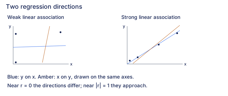
Two regression directions
Compare the fitted response on the same x-horizontal and y-vertical axes. These source-role sketches preserve illustrative points and lines, not numerical observations or regressions calculated from the drawing.
Weak linear association
- Solid: y on x
- Dashed: x on y
Strong linear association
- Solid: y on x
- Dashed: x on y
Keep the two response models distinct
The y-on-x fit minimises squared vertical residuals; the x-on-y fit minimises squared horizontal residuals on these axes. Rearranging one fitted equation does not generally produce the other fitted regression.
Both fitted lines pass through the means
For paired data with both variables varying, both least-squares regressions pass through this mean point. Use the actual observations or fitted equations to find it; the schematic positions supply no numerical mean.
At exactly zero linear correlation
When both variables vary and r is zero, both regression coefficients are zero. On the same axes, y-on-x is horizontal and x-on-y is vertical. The vertical line cannot be rewritten as a single-valued function y of x.
- Use the same axes and scale when comparing the two directions. A drawn angle is not a scale-independent measure of correlation; rescaling an axis changes the angle. Do not read a numerical r from these sketches.
- With perfect linear association and both variables varying, the fitted lines coincide. A constant variable makes the usual correlation coefficient undefined, rather than providing a zero-correlation example.
- Choosing a regression for prediction still depends on the prescribed explanatory role. Use the linked method to distinguish direct prediction from inverse calibration.
- Zero linear correlation does not rule out a nonlinear relationship. Inspect the scatter before accepting a line.
Compare with the source direction sketches
Expand diagramFit diagram to page
Use the scrollbars or arrow keys to inspect details.
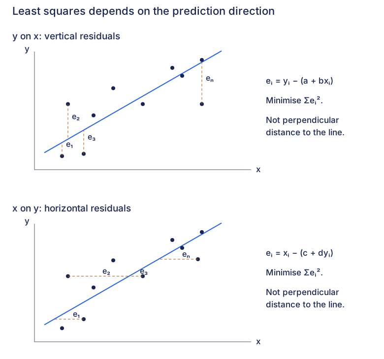
Vertical and horizontal residuals
Choose the response before measuring a residual. Both sketches keep x horizontal and y vertical. Their point positions and lines are schematic; they are not numerical data or fits calculated from those positions.
y on x: vertical residuals
Predict y from x
Keep the observed x coordinate fixed. The line supplies the predicted y response at that same input.
Measure the vertical residual
The residual is observed y minus predicted y. It is signed; the dashed segment shows its magnitude along the response coordinate.
Minimise squared vertical residuals
Choose a and b to minimise this sum over every observation. Squaring prevents positive and negative residuals from cancelling. The drawing marks four residual roles, not only four terms in the sum.
Compare each observation with its prediction.
- Ringed point: e₁.
e₁: below its prediction
The ringed observation lies below its prediction, so observed y minus predicted y is negative.
- Ringed point: e₂.
e₂: above its prediction
The ringed observation lies above its prediction, so observed y minus predicted y is positive.
- Ringed point: e₃.
e₃: below its prediction
The ringed observation lies below its prediction, so observed y minus predicted y is negative.
- Ringed point: eₙ.
eₙ: below its prediction
The ringed observation lies below its prediction, so observed y minus predicted y is negative.
x on y: horizontal residuals
Predict x from y
Keep the observed y coordinate fixed. The line supplies the predicted x response at that same input.
Measure the horizontal residual
The residual is observed x minus predicted x. It is signed; the dashed segment shows its magnitude along the response coordinate.
Minimise squared horizontal residuals
Choose c and d to minimise this sum over every observation. Squaring prevents positive and negative residuals from cancelling. The drawing marks four residual roles, not only four terms in the sum.
Compare each observation with its prediction.
- Ringed point: e₁.
e₁: right of its prediction
The ringed observation lies right of its prediction, so observed x minus predicted x is positive.
- Ringed point: e₂.
e₂: left of its prediction
The ringed observation lies left of its prediction, so observed x minus predicted x is negative.
- Ringed point: e₃.
e₃: right of its prediction
The ringed observation lies right of its prediction, so observed x minus predicted x is positive.
- Ringed point: eₙ.
eₙ: right of its prediction
The ringed observation lies right of its prediction, so observed x minus predicted x is positive.
- Changing the response changes the least-squares problem. Rearranging one fitted equation does not generally give the other fitted regression.
- Measure along the response coordinate, not perpendicular to the line. A residual may be positive, negative or zero; its square is nonnegative.
- The two source panels have distinct schematic observations. Do not treat them as numerical fits of one shared dataset, or calculate coefficients or residual totals from their drawing coordinates.
- The two sums measure errors in different response coordinates and may have different units. Compare candidate fits for the same response on the same observations; do not rank y-on-x against x-on-y by their raw residual totals.
Compare with the source residual sketches
Expand diagramFit diagram to page
Use the scrollbars or arrow keys to inspect details.
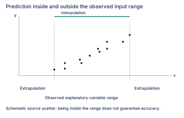
Interpolation and extrapolation
For direct prediction of a response y from an explanatory input x, compare the input with its observed range. This source illustration is schematic and supplies no numerical observations.
Below the observed inputs
Extrapolation. The explanatory input is smaller than every input observed in the sample.
Within the observed input range
Interpolation. The input lies between the smallest and largest observed inputs, including the limits.
Above the observed inputs
Extrapolation. The explanatory input is larger than every input observed in the sample.
- Check the explanatory-variable range. For a y-on-x prediction, compare the known x input with its observed x range, rather than with the response y range.
- Being inside the range does not guarantee accuracy. Check that the scatter supports the model; two observations alone cannot establish an underlying linear relationship.
- Keep the population and measurement context relevant. A strong correlation within a sample does not establish that the relationship continues outside the observed inputs.
Compare with the source range sketch
Expand diagramFit diagram to page
Use the scrollbars or arrow keys to inspect details.
Explore
Use the chemical-and-bacteria data in Review 2. Fit y on x and then x on y. Draw the residuals in the response direction for each fit: vertical for y on x, horizontal for x on y. Explain why each line minimises a different sum of squared discrepancies, so rearranging one fitted equation generally does not produce the other.
For the comparison requested in the question, refit without the suspect observation and inspect both the scatter and correlation again. In an investigation, excluding an observation needs a reason beyond improving the coefficient. Explain why correlation alone cannot establish a suitable model or a causal explanation, and check whether a proposed prediction stays inside the observed range.
Worked example
For , both sample means are 2.5. A calculator gives for y on x and for x on y, with . The first minimises squared y residuals and the second squared x residuals. At y=3, the reverse fit estimates x as , whereas rearranging the forward line gives . The different estimates reflect different fitting objectives. These are observational predictions, with the response chosen for the modelling task.
Inspect the scatter, residual direction and modelling setup. A large correlation does not establish causation or justify extrapolation, and rearranging a fit does not generally refit the other response.
Check your understanding
An observational dataset has , , , and , where S denotes centred sums. Observed x values span 2 to 8 and y values span 12 to 28. Find both regression lines. Choose the appropriate fitted line to estimate y when x=7 and x when y=24. Compare the latter estimate with rearranging the other line, and assess a prediction at x=20.
The y-on-x slope is , giving , or . The x-on-y slope is , giving , or .
For x=7, the y-response fit estimates y as 24. For y=24, the x-response fit estimates x as 6. Rearranging the forward fit would give , which does not minimise the x residuals. Both requested explanatory values lie inside their respective observed ranges, but interpolation still does not guarantee an accurate individual outcome. At x=20 the forward prediction would be extrapolation and needs additional model justification.
Mastery learning objectives
At the end of this chapter, I should be able to:
Choose a practice question
The source groups practice by skill. Its reference labels are retained below; each link opens the full exercise so you can locate the named part.
| Skill | Lecture examples | Discussion questions | Review follow-up |
|---|---|---|---|
| Calculate the r-value | 2(ii), 5(i), 8(i), 9(i), 10(ii)(iii), 11(ii) | 1 (1st part), 2(i), 3(iv), 4(b)(ii), 6(a)(ii), 8(f) | 1, 2(i), 3(ii), 4(i)(iv), 5(iii), 6(ii), 7(ii)(iii), 8(b)(ii), 9(ii) |
| Sketch a scatter diagram | 1 (1st part), 2(i), 3(iii), 10(i), 11(i) | 2(i), 3(i), 4(a) & (b)(i), 5(i), 6(a)(i), 7(ii), 8(d) | 1, 2(ii), 3(i), 4(i), 5(i), 6(i), 7(ii), 8(a) & (b)(i), 9(i) |
| Comment on the relationship using r, the scatter diagram and/or context | 1 (2nd part), 2(i), 10(i)(ii), 11(iii) | 1 (last part), 3(iv), 5(ii)(iii), 6(a)(iii), 7(ii), 8(a) | 1(i), 3(i)(a)(b), 4(i), 5(ii), 6(ii), 7(iv), 8(b)(ii) |
| Obtain a regression equation | 3, 5(ii), 8(ii) | 2(iii), 3(iii), 4(b)(iii), 5(iv), 7(iii), 8(f) | 1(ii), 2(i), 3(iii), 4(iii), 6(iii)(iv), 7(iii), 8(b)(iv), 9(ii)(iii) |
| Determine a variable using an appropriate regression and/or assess prediction validity | 7, 8(iv), 11(iv) | 3(v)(vi), 4(iv)(v), 6(a)(iv), 7(iii), 8(g) | 2(iv), 3(iv)(vi), 4 (1st part), 5(iv), 6(v), 7(v), 8(b)(v) |
| Identify outliers and perform necessary calculations | 2(iii), 5(iii) | 8(c) | 2(iii)(iv), 3 |
| Explain in context why strong correlation does not imply causation | — | 2(ii), 6(a)(v) | 4(ii) |
| Use the fact that a regression line passes through the mean point | 3 (last part), 4, 8(iii) | 3(ii), 6(b), 7(i) | 4(v), 7(i) |
| Use invariance of r under changes of measurement scale | 9(ii) | 7(v), 8(b) | 3(v), 8(b)(iii) |
| Use the sum of squared residuals | 6 | 8(e) | — |
Source-map notes: the prediction row prints Discussion “4(iv)(v)”; these refer to the age/earnings question’s (b)(iv)(v).
The printed Review “4 (1st part)” is preserved as source shorthand; open its full prompt to identify the requested task.
The final row names Discussion8(e); Discussion9(i)(b)–(d), (ii)–(iii) also directly practises residuals and squared-error comparison. This last suggestion is an authored extension to the printed map.
Positive rescaling leaves r unchanged; multiplying only one variable by a negative scale reverses its sign.
Practice questions
Practice section 1 · Questions 1–6
Identify explanatory and response variables · Sketch the eleven insulin and time observations · +4 more
Practice section 2 · Questions 7–12
Compare two scatters and fit both regression directions · Compare two models using squared residuals · +4 more
Practice section 3 · Questions 13–18
Compare linear and squared-speed models of drag · Calculate correlation from six summary values · +4 more
Practice section 4 · Questions 19–24
Compare pollution models and audit a damaged regression fragment · Recover a missing price index and choose the prediction direction · +4 more
- Compare pollution models and audit a damaged regression fragment
- Recover a missing price index and choose the prediction direction
- Compare used-car prices with reciprocal mileage
- Compare fuel-consumption models using squared residuals
- Choose a model with a limiting daily rate
- An outlier reverses the fitted trend
Practice section 5 · Questions 25–30
Refit a logarithmic model after finding a recording error · Transform PSI and recover an additional observation · +4 more
Practice section 6 · Question 31
Compare a linear trend with a transformed quadratic
Ready to try this on your own?
For “Correlation and linear regression”, try a question without the working and explain your method. This records your confidence, saved in this browser only.