Model and analyse recurrences

Generate a recurrence before justifying its behaviour

Example 30 models geese on a poultry farm, allowing for influences such as sales and deaths, by $u_{n+1}=0.75u_n+80$. Here $u_0$ is the initial population, so the calculator setup uses nMin=0, u(n+1)=0.75u(n)+80 and either u(0)=576 or u(0)=320. The requested first four updates are:

The source screens continue with these displayed values:

Later screen values are rounded displays of the real-valued model; retain unrounded intermediate values when calculating. The lecturer explicitly stresses “appears to be”: these first five values suggest a decreasing sequence in the first case and a constant sequence in the second. A short table alone does not justify behaviour for every index.

Unfold the same recurrence backwards or forwards

The source gives two derivations for Example 30. Starting from $u_n$, repeatedly replace the preceding term:

$$\begin{aligned} u_n&=0.75u_{n-1}+80\\ &=0.75(0.75u_{n-2}+80)+80\\ &=0.75^2u_{n-2}+80(1+0.75)\\ &=0.75^3u_{n-3}+80(1+0.75+0.75^2). \end{aligned}$$

Continuing for $n$ updates gives $0.75^nu_0$ plus $80$ times a GP with first term 1, ratio 0.75 and $n$ terms. Starting instead from $u_0$, expand successive updates:

$$\begin{aligned} u_1&=0.75u_0+80,\\ u_2&=0.75(0.75u_0+80)+80\\ &=0.75^2u_0+0.75(80)+80,\\ u_3&=0.75[0.75^2u_0+0.75(80)+80]+80\\ &=0.75^3u_0+0.75^2(80)+0.75(80)+80. \end{aligned}$$

The same constant contributions now appear in descending powers. Both methods reach

$$\begin{aligned} u_n&=0.75^nu_0+80\sum_{j=0}^{n-1}0.75^j\\ &=0.75^nu_0+80\frac{1-0.75^n}{1-0.75}\\ &=0.75^nu_0+320(1-0.75^n)\\ &=0.75^n(u_0-320)+320. \end{aligned}$$

The finite sum here is for $n\ge1$; the closed formula also gives $u_0$ at $n=0$. Since $0.75^n\to0$, $u_n\to320$.

For $u_0=576$, the distance above 320 is $256(0.75^n)>0$ and strictly decreases; indeed $u_{n+1}-u_n=-64(0.75^n)<0$.

For $u_0=320$, the coefficient of the power is zero, so $u_n=320$ for every integer $n\ge0$.

This formula justifies the earlier observations, as the second lecturer note requests.

A stray $u_4=320$ beneath the Student general derivation belongs only to the constant initial case; it is not true for every initial population.

Fit an explicit form and sum its three components

Example 31 is self-reading. The recurrence $u_{n+1}=2u_n+An$ and values $u_1=5,u_2=15$ give

$$15=2(5)+A\quad\Longrightarrow\quad A=5,\qquad u_3=2(15)+5(2)=40.$$

The Student copy explicitly supplies the $u_3$ update. Fit the given form $u_n=a2^n+bn+c$ with those three values:

$$\begin{aligned} 2a+b+c&=5,\\ 4a+2b+c&=15,\\ 8a+3b+c&=40. \end{aligned}$$

The source uses a calculator simultaneous-equation solver, obtaining $a=15/2,b=-5,c=-5$. Subtracting consecutive equations also gives $2a+b=10$, $4a+b=25$ and hence $2a=15$, which confirms the result.

For the sum, separate the geometric, arithmetic and constant pieces:

$$\begin{aligned} \sum_{r=1}^{n}u_r &=\sum_{r=1}^{n}\left[\frac{15}{2}(2^r)-5r-5\right]\\ &=\frac{15}{2}\sum_{r=1}^{n}2^r-5\sum_{r=1}^{n}r-5\sum_{r=1}^{n}1\\ &=\frac{15}{2}\left[\frac{2(2^n-1)}{2-1}\right] -5\left[\frac n2(n+1)\right]-5n\\ &=15(2^n-1)-\frac{5n}{2}(n+1)-5n. \end{aligned}$$

Each group contains $n$ terms. The geometric powers $2^1,2^2,\ldots,2^n$ start at 2 and have ratio 2; the natural numbers start at 1 and have difference 1.

The source labels say GP first term 1 and AP difference 2, but its following calculation uses the correct values.

The Teacher asks for the answer in terms of $n$; the Student prints “in terms of $u_1$”, although $u_1$ is already fixed at 5. Follow the Teacher’s variable and the worked answer; no further simplification is required.

Separate possible limits from observed convergence

Example 32 uses the graph of $h(x)=e^x-3x$. It has a positive intercept $h(0)=1$, two positive roots $\alpha<\beta$, and one minimum. It is negative between the crossings and positive outside them.

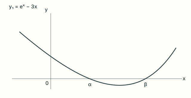
The calculator gives $\alpha\approx0.619$ and $\beta\approx1.512$ to three decimal places. Keep more digits when iterating or comparing values near a root. For the recurrence $x_{n+1}=e^{x_n}/3$, part (ii) assumes convergence. If $x_n\to L$, the shifted sequence also tends to $L$, and continuity gives

$$L=\frac13e^L\quad\Longrightarrow\quad3L=e^L \quad\Longrightarrow\quad e^L-3L=0 \quad\Longrightarrow\quad L=\alpha\ \text{or}\ L=\beta.$$

The source callout specifically explains this conditional instruction. The calculation identifies possible finite limits; it does not prove that every starting value converges. Retain the hypothesis in the concluding sentence.

For part (iii), the source calculator table displays:

A dash represents a blank cell in the source, not a zero or a failed calculation. Iterate unrounded values; repeated displayed values 0.619 do not mean exact equality with the root. The reported behaviours are increasing convergence to $\alpha$ from 0, decreasing convergence to $\alpha$ from 1, and increasing divergence from 2. The next sign analysis explains them.

Use a difference graph and preserve the relevant interval

For Example 32(iv), consider the difference asked for:

$$x_{n+1}-x_n=\frac13e^{x_n}-x_n =\frac13(e^{x_n}-3x_n).$$

The source suggests entering Y1=e^X−3X and Y2=(e^X−3X)/3. The second curve is a vertical compression of the first, retaining both roots and every sign:

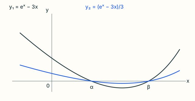
Between the roots the difference is negative; outside them it is positive:

$$\begin{aligned} \alpha<x_n<\beta&\Longrightarrow x_{n+1}-x_n<0 \Longrightarrow x_{n+1}<x_n,\\ x_n<\alpha\ \text{or}\ x_n>\beta&\Longrightarrow x_{n+1}-x_n>0 \Longrightarrow x_{n+1}>x_n. \end{aligned}$$

The source uses these graph signs. An algebraic check is $h''(x)=e^x>0$, while $h'(x)=e^x-3$ vanishes only at $x=\ln3$: the graph decreases to one minimum and then increases, giving the stated sign regions around its two roots.

For part (v), the source compares $0<\alpha$, $\alpha<1<\beta$ and $2>\beta$. To apply the sign result repeatedly, also check that later terms stay in the relevant region. The function $g(x)=e^x/3$ is strictly increasing and fixes $\alpha,\beta$, so

$$\begin{aligned} 0\le x<\alpha&\Longrightarrow x<g(x)<\alpha,\\ \alpha<x<\beta&\Longrightarrow\alpha<g(x)<x,\\ x>\beta&\Longrightarrow g(x)>x>\beta. \end{aligned}$$

Thus the sequences starting at 0 and 1 are respectively increasing/bounded above and decreasing/bounded below. Their finite limits must be $\alpha$.

The sequence starting at 2 increases and stays above $\beta$.

If it had a finite limit, that limit would be at least 2, contradicting the only possible limits in (ii); hence it is unbounded and tends to positive infinity.

This interval/boundedness reasoning supplies the detail behind the observed behaviours. Increasing alone does not imply divergence.