Probability and conditional information
← Back to lesson · Complete chapter reading and print view · Open reference notes separately
By the end, you can
- Use complements, unions and intersections
- Distinguish independence from mutual exclusivity
- Calculate conditional probabilities using the right reference set
about 40 minutes for the lesson · practise at your own pace.
The central idea
What this chapter counts
The source outline covers addition and multiplication of probabilities, mutually exclusive and independent events, outcome tables, Venn and tree diagrams, counting with permutations and combinations, and conditional probabilities. Its three headline identities are the complement rule, the two-event addition rule, and the conditional probability formula.
The opening dice question below introduces probability through a gambling puzzle. The notes connect it to mid-seventeenth-century correspondence involving Blaise Pascal and Pierre de Fermat, then name quantum mechanics, gas kinetics, insurance risk and genetics as applications. The original dice photograph is decorative; the two mathematical events are retained in the activity.
Define the sample space and the event
An experiment generates data. An observation records numerical or categorical information. A sample space S is the set of all possible outcomes; it may be finite or infinite. Each outcome is a sample point, element or member of S. Outcomes are equally likely when they have equal chances. An event E is a subset of S.
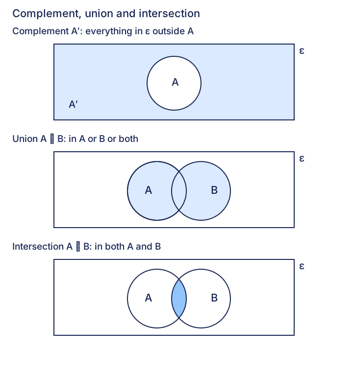
Relative to a universal set ε, is the complement of A; contains elements in A or B or both; contains elements in both. The empty set is or , and n(A) is the number of elements in A. In a probability problem the universal outcome set is S.
For a fair coin, H and T denote a head and a tail. Three tosses give the finite sample space . Tossing repeatedly until a tail gives the infinite stopping-string space .
| Event | Three tosses | Stop at the first tail |
|---|---|---|
| A tail is observed once | All of S | |
| Tails are observed at least twice | ||
| Heads are observed three times |
The stopping strings have probabilities 1/2,1/4,1/8,…, not equal weights. This model records completed stopping strings; endless heads has probability zero under independent fair tosses. The source phrase “drawn at random means all outcomes are equally likely” describes its intended uniform finite-selection model. Randomness by itself does not guarantee uniform probabilities.
Count only when elementary outcomes are equally likely
For a finite, nonempty sample space of equally likely outcomes,
The source’s function note views probability as a map from events, which are subsets of the outcome space, to numbers in [0, 1].
The seven printed results and their reasoning are:
- If , then , so .
- If E=S, then n(E)=n(S), so .
- Since , . Divide by n(S)>0 to obtain .
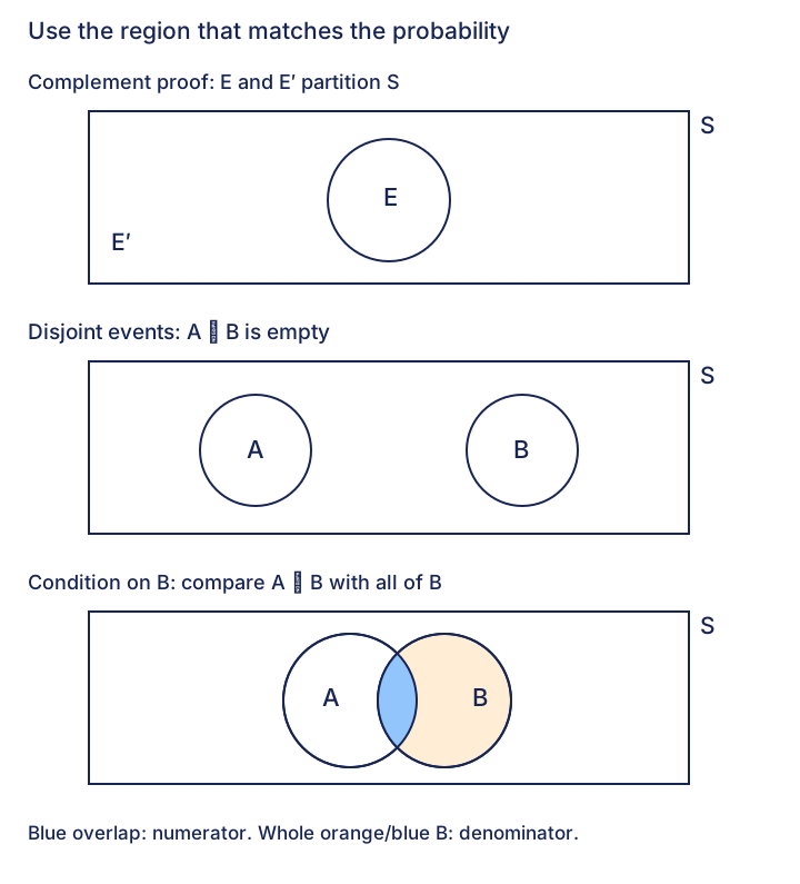
- E and E′ partition S: . Divide by n(S) to get , hence .
- Adding P(A) and P(B) counts the overlap twice. Subtract one copy: .
- Intersection is symmetric: .
- Union is symmetric: .
Recognise mutually exclusive events
Mutually exclusive events have no common outcomes: , so . For one die roll, getting 1 and getting 2 are mutually exclusive. Getting 1 and getting an odd number are not: outcome 1 is shared. The notes acknowledge OpenIntro Statistics, second edition for this explanation.
Substitute the zero overlap into the addition rule:
For pairwise mutually exclusive , .
The source tests mutual exclusivity through either zero intersection probability or equality in the addition formula. These are equivalent to an empty intersection in the finite positive-probability elementary-outcome model used here. In general probability spaces, zero probability need not mean an empty set; the set definition remains no shared outcomes.
Change the reference set when information is given
John rolls a fair die and Peter guesses its result. A specified number has probability 1/6. Given that the result is even, the possible outcomes reduce from {1,2,3,4,5,6} to {2,4,6}, and each has conditional probability 1/3.
Mary’s class has 25 students: 15 boys and 10 girls. Selecting one student uniformly gives Mary probability 1/25. Given that a girl was selected, the reference set is the 10 girls and Mary’s probability becomes 1/10. This concrete example applies the same change of denominator.
For P(B)>0,
In a finite equally likely model, the source proves this by dividing the favourable and reference counts by n(S):
The source assumes both P(A)≠0 and P(B)≠0 in its introduction; only P(B)>0 is required to define P(A|B). The reverse conditional P(B|A) additionally needs P(A)>0.
If A and B are mutually exclusive and P(B)>0, then . Rearranging gives . Similarly , so, when both conditionals are defined,
The source deck illustration is retained using labelled suits and ranks. Its printed illustration credit is the card-image source; this is a provenance pointer, not additional course content.
Test independence using the probability model
Two events are independent when learning that one occurred does not change the probability of the other. The source example combines a coin toss and a die roll: knowing the coin is heads does not change the probability that the die is odd, assuming the two processes operate independently. This is a statement about probabilities, not a claim about causation.
Where the conditionals exist, independence gives and . Substituting the first equality into the conditional formula gives , hence
The source lists three equivalent tests: either conditional equality when defined, or the product equality. The product test also works when an event has probability zero. For mutually independent , . Here independent means mutual independence; pairwise independence alone is not enough for that general product.
Complementing independent events preserves independence
If A and B are independent, so are A′ and B, A and B′, and A′ and B′. The source gives two full proofs and asks you to prove the remaining case in the activity below.
For A′ and B, start with the region in B outside A:
For both complements, use the complement of the union and factor:
Try the analogous proof for A and B′ before opening its working. Example 3 then tests independence and mutual exclusivity separately, and Self-Practice 3 requires recovering all of A from its portions inside and outside B.
Choose a problem-solving tool
| Approach | When it is useful |
|---|---|
| Table of outcomes | Two components and a small sample space. |
| Venn diagram | Multiple events, intersections and complements, such as and . |
| Permutations and combinations | Selection without replacement or arrangement. |
| Tree diagram | A series of experiments or sequential events. |
Example 4 constructs a complete 6×6 table for two throws, with the first throw across columns and the second down rows. Every ordered cell is equally likely; the displayed sums are not equally likely. Use the table for the intersection numerator, then choose the probability of the given event as denominator.
The source recommends the conditional probability formula.
Its alternative counting method first identifies the reduced reference space, then the favourable outcomes inside it. The Teacher guidance highlights these in that order.
Count ratios require equally likely elementary outcomes in the reference space; a reduced space being easy to list is a practical convenience.
The source repeats the same table for several methods; the native four-panel diagram retains all 36 cells and each distinct highlighted reference/favourable set.
Subtract sets before substituting probabilities
Venn diagrams make a region subtraction visible. In Example 5, the union is partitioned into B and A-only, so . This is the Teacher’s visual subtraction argument. Once B is known, independence replaces by P(A)P(B) in the addition formula to find A.
For , identify the excluded region: B-only, or . The Teacher diagram splits B into its overlap with A and its part outside A. Subtract the overlap from B, then complement the result. Source circle areas are schematic and do not encode the numerical probabilities.
Keep the counting model consistent
For uniformly chosen finite outcomes, probability is favourable count divided by total count. With repeated letters, the numerator and denominator must describe the same distinct-arrangement model. SEPTEMBER has three identical Es; PROBABILITY has two Bs and two Is. Uniform shuffling of the physical copies gives every distinct arrangement the same number of labelled-copy realisations, justifying the ratio.
For three copies, not all together and all separated are different events. The Teacher’s SEPTEMBER warning is explicit: the former includes a pair together and a third copy elsewhere. For two copies, the complement of together is separated.
Read every tree branch relative to its preceding path
A probability tree traces sequential events. The first split is A or A′. Each of those nodes then splits into B or B′. The four complete path probabilities are:
Each branch probability is conditional on the path so far; the first split is conditional on the initial sample space. Sibling alternatives from a reached node are mutually exclusive and exhaustive, and their probabilities sum to 1. This is the intended meaning of the source’s “nodes from the same branch” wording.
Multiply along a complete path; add disjoint complete paths for an event.
For a zero-probability preceding event, its ordinary conditional is undefined and that path contributes zero without needing a ratio there.
The source’s diagram note explains that Venn and tree diagrams present sample spaces, relationships between sets and event outcomes, helping calculate probabilities. Example 7 models two counters without replacement using both a sequential tree and combinations of distinct physical counters. The two methods use different but internally consistent elementary outcomes and agree on all three answers.
Add disjoint paths before conditioning on the result
Example 8 first divides customers by fuel type, then by whether they fill their tanks. To find a not-full tank, multiply along each of the three not-full paths and add them: the fuel categories are disjoint and exhaustive. To condition on a full tank, divide the desired fuel-and-full probability by the total probability of a full tank, including all fuel types.
Self-Practice 7 uses the same structure with machine identity and defect status. Production shares weight the three conditional defect rates. Independence of defects across different items does not mean that a machine’s identity and defect status are independent for the selected item.
Replacement keeps the composition fixed
In Example 9, replacement keeps the blue/white proportions unchanged between draws. For independent random draws, the joint probability factors into the two one-draw probabilities. The Teacher guidance therefore uses direct multiplication instead of a tree.
For an inclusive union, either add disjoint outcome cases or subtract the complement. “First blue or second white” includes BW, BB, WW and excludes only WB. This retains both source methods while making the overlap explicit.
Prefer a compact count when a full tree becomes large
Example 10 first uses a complete 27-path tree for three replacement draws. Its six all-different colour orders all have the same probability 0.03, so one path probability multiplied by 3! gives 0.18. The Teacher recommends this compact order count rather than teaching a lengthy tree construction. The complete native tree remains available for comparison.
Without replacement, repeated draw probabilities change with the remaining supplies.
The same example retains both source approaches: a probability for one colour order multiplied by its number of distinct orders, and an unordered selection count using distinct physical balls. The source’s 3^5=243 candidate-colour-string remark includes strings that would exhaust a colour and have zero probability.
It is not a uniform sample space.
In the six-path symbolic sum, the printed G1,W1,R2 indices are qualified as the intended G1,W2,R3 path.
Identify the repeat unit in a geometric progression
Example 11 restarts only after a complete round in which A, B and C all fail. The repeat probability is therefore (5/6)^3, not 5/6. The source case table counts A’s own attempts; each successive winning opportunity adds another full failed round. Sum the disjoint winning cases using an infinite geometric progression.
Example 12 counts at least one dart success in n throws, either by complementing all n misses or by summing first-hit cases 1 through n.
Once a hit occurs, later outcomes do not alter that event, as the Teacher notes emphasize.
Use the finite geometric sum or the complement expression, retain the strict threshold, reverse the inequality on dividing by a negative logarithm, and confirm the least integer with the source calculator table.
Complement, union and intersection
Expand diagramFit diagram to page
Use the scrollbars or arrow keys to inspect details.
Complement, disjointness and conditional reference sets
Expand diagramFit diagram to page
Use the scrollbars or arrow keys to inspect details.
Read a two-stage probability tree
Explore a probability tree
Choose outcomes, change conditional probabilities, and compare path products with event totals.
Multiply along a complete path; add disjoint complete paths. Each reached split totals 1. Second-stage probabilities are conditional on the first event.
Explore
For 10,000 modelled items, compare defective rates of 1% and 10%. In both populations a scanner flags 90% of defective items and 5% of nondefective items. Predict how the defective share among flagged items will change before building expected-count tables. Label the conditioning group in every fraction, and check the result using disjoint paths in a tree. Explain why a flag rate among defective items cannot simply be reversed.
Worked example
A bag contains three red and two blue balls. Drawing twice without replacement gives . Given that the first was red, the second-red probability is , not .
Mutually exclusive events with positive probabilities cannot be independent.
Check your understanding
Box A contains three red and one blue counter; box B contains one red and five blue counters. Choose a box with equal probability, then draw two counters from that box without replacement.
Find the probability of two reds and, given two reds, the probability that box A was chosen.
Compare with drawing two counters without replacement after pooling all ten counters.
Explain why the sampling mechanisms give different answers.
Let R mean two red draws. From A, ; from B it is zero. Hence and .
The pooled experiment has four red counters among ten, so its two-red probability is . Choosing a box equally does not select individual counters uniformly when the box sizes differ. It also makes both draws share the chosen box. The probability model must follow the actual selection mechanism and update the composition after the first draw.
Mastery learning objectives
At the end of this chapter, I should be able to:
Choose a practice question
Use the printed question-type map to choose a method to practise. Each link opens the complete question; the printed part references are retained.
| Skill | Lecture examples | Discussion | Review follow-up |
|---|---|---|---|
| Mutually exclusive events | 1, 3(ii) | 2(last part) | — |
| Independent events | 3(i) | 2(last part), 6(iv) | 1, 2, 4(iii)(iv), 6(i) |
| Table of outcomes | 4 | 1 | — |
| Venn diagrams | 5 | 2(i), 6 | 4, 5, 6(ii) |
| Permutations and combinations | 6, 9, 10 | 3, 4, 7 | 9, 10, 11, 14(a), 16 |
| Tree diagrams | 7, 8 | 5, 8 | 8, 12, 13, 14(b), 15 |
| Conditional probabilities | 2, 3, 4(iii)(iv), 7(iii), 8(iii), 10(c) | 1(v), 2(ii)(iii), 5(a)(iv) & (b), Q6(iii), Q8(ii) | 2, 3, 4(i)(ii), 6(i), 8(iii), 9(ii), 11(iii), 12(i), 13(i) & (ii)(b), 14(b)(ii), 15(ii), 16(ii) |
| Prior topic: geometric progression | 11, 12 | 7(iv) | — |
| Prior topic: applications of differentiation | — | 8(last part) | — |
| Future topic: binomial distribution | — | — | 12(iii) |
Check the part reference against the question. The conditional-probability reference Example 10(c) means 10(ii)(c).
The future-topic row prints Review 12(iii), but Review 12 has an initial unnumbered ask followed by (i) and (ii); its repeated-match calculation is (ii). The link opens that complete question.
Example 9 is listed under permutations and combinations although its printed solution uses direct replacement probabilities. Keep the source pointers while choosing the method from the actual question.
Practice questions
Practice section 1 · Questions 1–6
Compare the two opening dice events · Can one match have two incompatible goal totals? · +4 more
Practice section 2 · Questions 7–12
Distinguish dependence from a nonempty overlap · Find P(A) before testing independence · +4 more
Practice section 3 · Questions 13–18
Distinguish separated Es from not all Es together · Arrange PROBABILITY with adjacent or separated Is · +4 more
Practice section 4 · Questions 19–24
Use order counts instead of expanding every draw path · Sum the chances of winning on successive rounds · +4 more
- Use order counts instead of expanding every draw path
- Sum the chances of winning on successive rounds
- Find the least dart count for a strict probability target
- Two throws: ordered outcomes and conditioning
- Recover a marginal probability from a conditional one
- Use the same equally likely four-person selections throughout
Practice section 5 · Questions 25–30
Distinguish not-all-together from pairwise separation · Use base rates before interpreting a positive result · +4 more
- Distinguish not-all-together from pairwise separation
- Use base rates before interpreting a positive result
- Use overlap bounds before adding the conditional information
- Sum mutually exclusive winning rounds as a geometric series
- Differentiate the posterior probability over its percentage domain
- Solve for a parameter and enforce probability bounds
Practice section 6 · Questions 31–36
Recover the marginal before testing independence · Link both conditional probabilities through the shared intersection · +4 more
- Recover the marginal before testing independence
- Link both conditional probabilities through the shared intersection
- Bound the part of C lying in B but outside A
- Recover A from a disjoint region before using independence
- Keep the two dice ordered when checking event independence
- Account for the first red ball being removed
Practice section 7 · Questions 37–42
Use the preceding meal to choose each transition probability · Condition a hypergeometric count on at least one match · +4 more
- Use the preceding meal to choose each transition probability
- Condition a hypergeometric count on at least one match
- Keep a grouped IP pair and separately place the JC2 members
- Condition on the first black draw before counting the remaining whites
- Separate dependent sets from independent repeated matches
- Give proper fractions and condition on both people finding jobs
Practice section 8 · Questions 43–45
Distinguish finite sampling from independent-person conditioning · Correct the intermediate expansion before solving for the percentage · +1 more
Ready to try this on your own?
For “Probability and conditional information”, try a question without the working and explain your method. This records your confidence, saved in this browser only.