Definite integrals, areas and volumes

A definite integral accumulates signed contributions and can be evaluated by F(b)−F(a) when F′=f under the fundamental theorem. Geometric area is nonnegative, so split where the curve crosses an axis or two curves exchange order. Revolving a region produces cross-sectional discs or washers; integrate their areas.

Rectangle sums and the limiting integral

Divide $[a,b]$ into n equal intervals of width $\Delta x=(b-a)/n$. Each rectangle has area height times width. With the source indexing $x_1=a$, $x_{n+1}=b$, left heights give $L_n=\sum_{i=1}^nf(x_i)\Delta x$ and right heights give $R_n=\sum_{i=1}^nf(x_{i+1})\Delta x$.

For continuous f, both sums tend to $\int_a^bf(x)\,dx$ as $n\to\infty$ and $\Delta x\to0$. The finite expressions are Riemann sums; their limit is the integral. For the source curve above the axis, that limit is area A. Signed integrals need care when a curve crosses the axis.

The teacher annotations emphasise total rectangle area and taking a limit. Left endpoint i is $a+(i-1)\Delta x$; the handwritten alternative $a+i\Delta x$ is its right endpoint. Sketch the region before selecting bounds, differences of areas or a solid of revolution.

The source’s historical note identifies Georg Friedrich Bernhard Riemann, a German mathematician of the nineteenth century. Its “Limits” callout links limits to the development of calculus and area under a curve; its “Diagrams” callout recommends sketching before identifying areas, formulating integrals or modelling a solid of revolution. The Teacher shades endpoint rectangles, underlines height times width and highlights the limiting step.

The source calls the displayed limit a “Riemann Sum”; here the finite sum is the Riemann sum and its limit is the definite integral.

Its right-endpoint diagram is followed by a printed $\sum f(x_i)\Delta x$ expression using the earlier left indexing; keep $f(x_{i+1})$ for the right-endpoint sum with $x_1=a$.

Both converge to the same integral.

A finer partition converges for this continuous curve, but its approximation error need not decrease at every individual value of $n$.

Antiderivatives and the fundamental theorem

If $f$ is continuous on $[a,b]$ and $F'=f$, then $\int_a^bf(x)\,dx=[F(x)]_a^b=F(b)-F(a)$. The lower and upper limits are $a$ and $b$. For example, an antiderivative of $x^2$ is $x^3/3$; the arbitrary constant cancels in the subtraction.

Five useful properties

For continuous $f,g$ and constant $k$: $\int_a^af=0$; $\int_a^bf=-\int_b^af$; $\int_a^bf=\int_a^cf+\int_c^bf$ for $a<c<b$; $\int_a^b(f\pm g)=\int_a^bf\pm\int_a^bg$; and $\int_a^bkf=k\int_a^bf$. The source prints $k\ne0$ for the last rule, but it also holds for $k=0$.

Continuity on the whole interval matters for this version of the theorem. The source warns against evaluating $\int_{-1}^1x^{-2}\,dx$ by direct substitution: $x^{-2}$ is undefined at zero. Its improper integral diverges to positive infinity; a formal endpoint subtraction does not evaluate it.

Signed integrals and geometric area

For a nonnegative curve on $[a,b]$, $A=\int_a^bf(x)\,dx$. For a nonpositive curve, $A=-\int_a^bf(x)\,dx$. If the curve is above the axis from $a$ to $b$ and below it from $b$ to $c$, add positive areas: $A=A_1+A_2=\int_a^bf(x)\,dx-\int_b^cf(x)\,dx$. Sketch first, find every zero inside the bounds, and split wherever the sign changes.

For the source sine example, $\int_{-\pi}^0\sin x\,dx=-2$ and $\int_0^{\pi}\sin x\,dx=2$. Origin symmetry makes the two geometric areas equal to $2$ each. Their combined geometric area is $4$, while $\int_{-\pi}^{\pi}\sin x\,dx=0$.

The Teacher points out odd/even symmetry for integrals on $[-k,k]$. For continuous odd $f$, the integral is zero; for continuous even $f$, it is $2\int_0^kf(x)\,dx$. The additional cosine query is $\int_{-\pi}^{\pi}\cos x\,dx=2\int_0^\pi\cos x\,dx=0$. Its zero result comes from evaluation of the even-function half-interval integral, rather than odd symmetry.

Horizontal strips and integration with respect to y

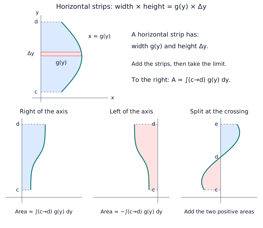
For a continuous curve $x=g(y)$, bounded by the y-axis and $y=c$, $y=d$, use horizontal strips. A strip has width $g(y)$ and height $\Delta y$, so its area is $g(y)\Delta y$ when $g(y)\ge0$. Adding strips and taking the limit gives $A=\int_c^dx\,dy=\int_c^dg(y)\,dy$ for a region to the right of the y-axis.

For a region to the left, $g(y)\le0$, use $A=-\int_c^dg(y)\,dy$. If the curve is left of the axis on $[c,d]$ and right on $[d,e]$, add the positive pieces: $A=A_1+A_2=-\int_c^dg(y)\,dy+\int_d^eg(y)\,dy$. Find the y-coordinate where the curve crosses the axis before splitting. Width, not height, is now the function of the integration variable.

Areas between curves

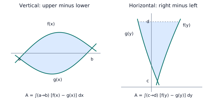
The source asks for the area between $y=f(x)$ and $y=g(x)$ from $a$ to $b$. In its first picture both are above the x-axis and $f(x)\ge g(x)$, so subtract the area $G$ under $g$ from the area $F$ under $f$: $A=F-G=\int_a^bf(x)\,dx-\int_a^bg(x)\,dx=\int_a^b[f(x)-g(x)]\,dx$.

The same upper-minus-lower strip width works anywhere in the plane, including below the x-axis. In that case do not describe each signed integral separately as an unsigned geometric area: the difference is the positive vertical distance. If the curves exchange order, find the crossings and split before adding areas.

For horizontal strips between $x=f(y)$ on the right and $x=g(y)$ on the left, use $A=\int_c^d[f(y)-g(y)]\,dy$. The summary rule is upper minus lower with x bounds, or right minus left with y bounds. Find the intersection coordinates to obtain the limits. A line is another curve, so the same rule applies; a triangle or trapezium can sometimes replace one of the simpler integrals.

Volumes as limits of disc sums

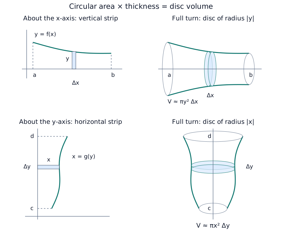
A complete rotation of a plane region about a line in its plane forms a solid of revolution; the line is the axis of revolution. For a nonnegative continuous $y=f(x)$ on $[a,b]$, rotate the region down to the x-axis through $360^\circ$ or $2\pi$ radians. Divide the interval into $n$ equal widths $\Delta x=(b-a)/n$. Rotating a rectangle creates a circular disc with radius $f(x_i)$ and thickness $\Delta x$. Its volume is $\pi[f(x_i)]^2\Delta x$, from circular area times thickness.

The finite disc sum is $V_n=\pi\sum_{i=1}^n[f(x_i)]^2\Delta x$. As $n\to\infty$ and $\Delta x\to0$, $V=\lim V_n=\pi\int_a^by^2\,dx=\pi\int_a^b[f(x)]^2\,dx$. The finite expression is a Riemann sum for volume; its limit is the integral. The Teacher highlights the squared radius and the limiting step.

For rotation about the y-axis, write $x=g(y)$ first and use horizontal strips of thickness $\Delta y$. A disc has radius $|x|$ and volume approximately $\pi x^2\Delta y$, so $V=\pi\int_c^dx^2\,dy=\pi\int_c^d[g(y)]^2\,dy$. The printed formula is correct; a nearby Teacher handwritten $\pi\int y^2\,dx$ does not match this y-axis setup and must not replace it. Match the radius, thickness variable and limits to the chosen axis.

Cylinders, cones and a translated axis

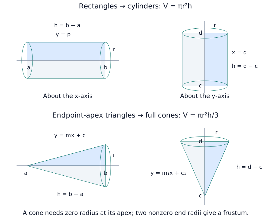
The source asks which solid is formed by rotating either (a) the rectangle between the x-axis, $x=a,b$ and $y=p$ about the x-axis, or (b) the rectangle between the y-axis, $y=c,d$ and $x=q$ about the y-axis. Both form a cylinder, with $V=\pi r^2h$. In (a), $r=|p|$ and $h=b-a$; in (b), $r=|q|$ and $h=d-c$ (bounds increasing).

It then asks about rotating a straight-line boundary $y=mx+c$ ($m\ne0$) about the x-axis, or $y=m_1x+c_1$ ($m_1\ne0$) about the y-axis. The drawn triangular regions form a cone, with $V=\frac13\pi r^2h$.

In the source drawings the radius vanishes at an endpoint, which is essential for a full cone.

The general straight-line wording needs this qualification: if both endpoint radii are nonzero on the same side, the solid is a frustum; if the line crosses the axis inside the interval, split the region instead of applying one cone formula indiscriminately.

For an axis parallel to a coordinate axis, translate the graph and its axis together until that axis coincides with x=0 or y=0. This preserves all radii and the generated volume, as in Example 16.

Washers between two curves

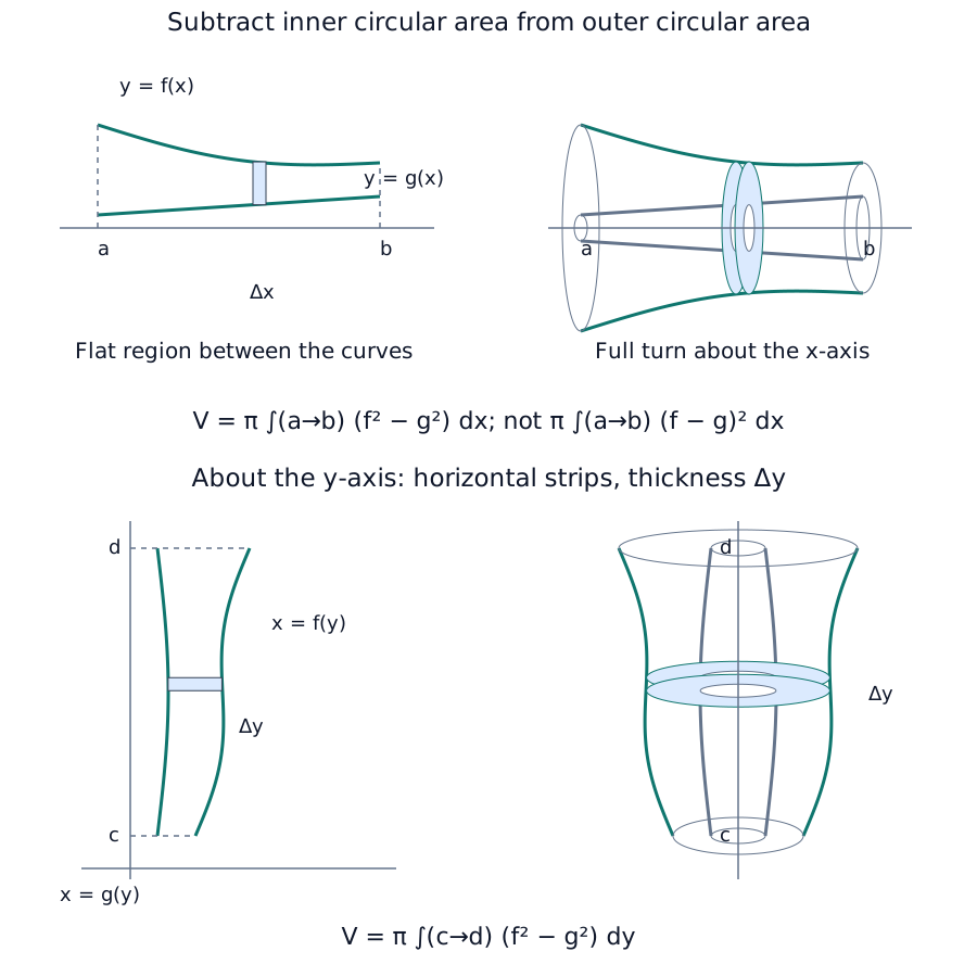
For $f(x)\ge g(x)\ge0$ throughout $[a,b]$, a full x-axis turn of the region between the curves gives outer radius $f(x)$ and inner radius $g(x)$. A washer has area $\pi[f(x)]^2-\pi[g(x)]^2$, so $V=\pi\int_a^b[f(x)]^2\,dx-\pi\int_a^b[g(x)]^2\,dx=\pi\int_a^b([f(x)]^2-[g(x)]^2)\,dx$. Subtract the inner solid from the larger one. This is not $\pi\int_a^b[f(x)-g(x)]^2\,dx$; square the two radii separately before subtracting.

For y-axis washers with $f(y)\ge g(y)\ge0$ on $[c,d]$, rotate the region between $x=f(y)$ and $x=g(y)$ through a full turn. Then $V=\pi\int_c^d[f(y)]^2\,dy-\pi\int_c^d[g(y)]^2\,dy=\pi\int_c^d([f(y)]^2-[g(y)]^2)\,dy$. The horizontal strip becomes an annular disc with thickness $\Delta y$.

The Teacher’s closing summary is: for the x-axis use $\pi\int y^2\,dx$ (or outer squared minus inner squared); for the y-axis use $\pi\int x^2\,dy$ (or the corresponding difference); for other parallel lines, translate region and axis together. Rewrite the radius in the chosen integration variable before comparing inner and outer boundaries.