Applications of differentiation
← Back to learning units · Complete chapter reading and print view · Open reference notes separately
By the end, you can
- Connect derivative signs to increasing and decreasing behaviour
- Classify stationary points and find tangents
- Model optimisation and connected rates
about 40 minutes for the lesson · practise at your own pace.
The central idea
The first derivative gives slope and the second describes how that slope changes. Stationary points satisfy f′(x)=0, but their nature needs a sign change or another test. In optimisation, reduce the quantity to one variable, preserve the physical domain, and compare candidates with boundaries. Connected rates differentiate a relation with respect to time.
Increasing versus strictly increasing
On an interval I, for every , increasing means and strictly increasing means . Decreasing and strictly decreasing reverse those inequalities to and .
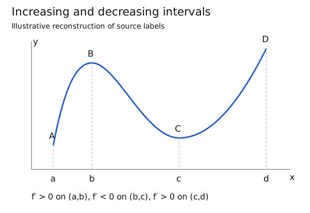
If f is differentiable and throughout I, f is strictly increasing there; a negative derivative throughout gives strict decrease. The source curve increases on and and decreases on . These are sufficient tests: strict increase can still allow an isolated zero derivative, as with at zero.
Why applications need a model
The source introduces uses in physics (motion, electricity, heat, light, harmonics, acoustics, astronomy and dynamics), chemistry (reaction rates and radioactive decay), biology (birth/death rates), economics (marginal cost/revenue and profit), engineering, statistics and medicine.
Its supermarket example asks how to choose the height-to-diameter ratio of a cylindrical can to minimise manufacturing surface area at fixed volume.
The original can photograph is retained in the source archive, with its printed DataGenetics attribution; the linked external page has not been reviewed.
The full chapter outline also includes interpreting first/second derivative signs, relating a function’s graph to its derivative’s graph, tangents/normals including implicit curves, calculator extrema, analytical classification, optimisation and connected rates. The complete lecture now connects these ideas through sixteen examples, three self-practices, source diagrams and the linked Discussion/Review questions.
Increasing and decreasing intervals
Expand diagramFit diagram to page
Use the scrollbars or arrow keys to inspect details.
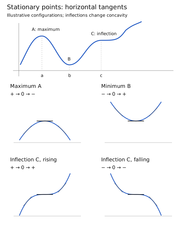
Method map: Classify a stationary point
Start at an interior input a where f′(a) = 0. Either test can establish a local maximum or minimum; an inconclusive test needs more information.
First-derivative test
Use signs that hold on small intervals on either side of a. Two isolated sample values are not a proof.
- Positive → zero → negativeLocal maximum
The curve rises into the point, then falls. Its value is greater than nearby values.
- Negative → zero → positiveLocal minimum
The curve falls into the point, then rises. Its value is less than nearby values.
- Positive on both sides, or negative on both sidesNo local extremum
There is no turning point. Confirm a change of concavity before calling this a stationary inflection; the same-sign pattern alone does not prove one.
These conclusions are local, not a comparison with the whole graph. If the one-sided signs do not settle, this chart is inconclusive; use another local argument.
Second-derivative test
At the same stationary input, apply the test under the usual local differentiability assumptions. This is an alternative test; you do not have to perform both tests.
- Negative second derivativeLocal maximum
establishes a strict local maximum.
- Positive second derivativeLocal minimum
establishes a strict local minimum.
- Zero or unavailable second derivativeInconclusive
Return to the first-derivative test or another valid local argument. A zero second derivative does not prove an inflection.
The worked comparisons below show three different outcomes with . Predict each outcome before opening its reasoning.
Find the point’s height by substituting a into f, not into a derivative. For an optimisation problem, compare valid candidates with relevant domain boundaries too.
Try a worked example
Read a case, make a prediction, then reveal the reasoning. The examples keep their stated values.
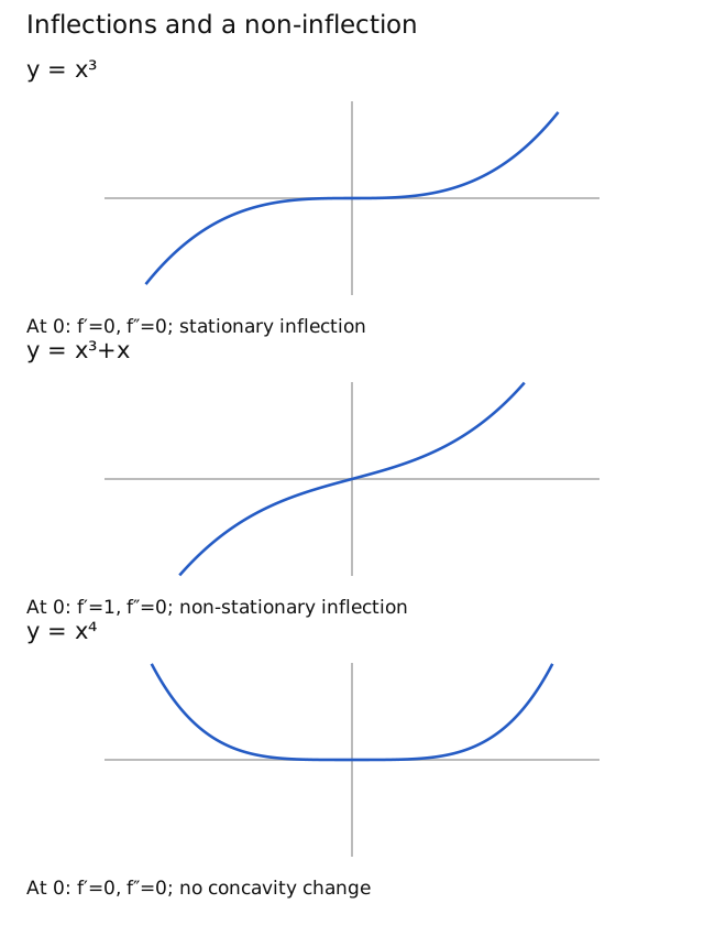
Compare the cubic at zero
For the illustrative function , classify the stationary point at . All three comparisons have : what extra evidence decides this one?
Show reasoning
1. Recognise the inconclusive test
The input is stationary, but a zero second derivative does not classify the point.
2. Check the signs on intervals
For every and every , . The curve is increasing on both sides, so the point is neither a local maximum nor a local minimum. These are interval statements, not just two sampled slopes.
3. Establish the change of concavity
The second derivative is negative to the left and positive to the right of zero. Concavity changes, and , so is a stationary point of inflection. Same-sign first derivatives alone would not establish the concavity change.
Compare the quartic at zero
For the illustrative function , classify the stationary point at . Does force the same outcome as the cubic? Predict the signs of on either side.
Show reasoning
1. Recognise the same inconclusive result
Both derivatives vanish at zero. The second-derivative test supplies no classification.
2. Use the first-derivative sign change
For every , ; for every , . The curve falls into the point and rises away, establishing a strict local minimum at . The height comes from , not from a derivative.
3. Check with the function values
Every nonzero nearby input has . This independently confirms the strict minimum. Also, on both sides: concavity does not change at zero, so this is not an inflection.
Reflect the quartic in the x-axis
For the illustrative function , classify the stationary point at . The second derivative is still zero there. Predict what reflecting the quartic does to its first-derivative signs.
Show reasoning
1. Keep the test's limitation
The negative sign changes the nearby slopes, but both derivatives at zero are still zero.
2. Reverse the sign change
For every , ; for every , . The curve rises into the point and falls away, establishing a strict local maximum at .
3. Check the value and concavity
Every nonzero nearby input has . The second derivative is negative on both sides, so concavity does not change. Across the three comparisons, the same zero second derivative permits an inflection, a minimum or a maximum.
Compare with the curve sketches
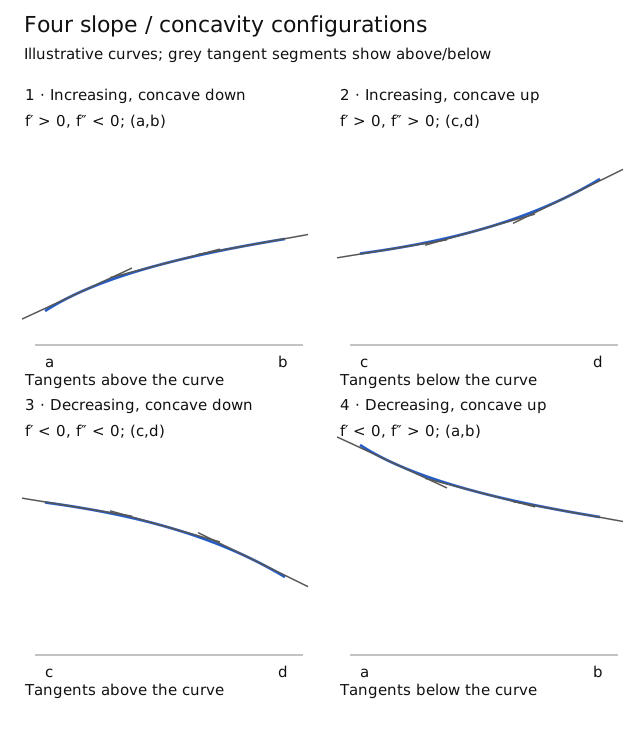
Compare the four local configurations below. All four functions are defined for every real x; each plot shows only the stated window. These functions illustrate the source’s four cases, not equations inferred from its combined A/B/C sketch.
Local maximum: rising, then falling
. Inspect around the stationary point .
- Left of the point
On , : rising.
- At the point
. Horizontal tangent .
- Right of the point
On , : falling.
Since , these signs hold throughout the stated intervals. They establish a strict local maximum at . Also . The full cubic is unbounded above, so this is not a whole-graph maximum.
Local minimum: falling, then rising
. Inspect around the stationary point .
- Left of the point
On , : falling.
- At the point
. Horizontal tangent .
- Right of the point
On , : rising.
The factorisation establishes these signs on whole intervals, giving a strict local minimum at . Also . The full cubic is unbounded below, so this is not a whole-graph minimum.
Stationary inflection: rising on both sides
. Inspect around .
- Left of the point
On , .
- At the point
. Horizontal tangent .
- Right of the point
On , .
There is no turning point. To establish an inflection as well, check : it is negative to the left and positive to the right, so concavity changes. The zero value alone is inconclusive.
Stationary inflection: falling on both sides
. Inspect around .
- Left of the point
On , .
- At the point
. Horizontal tangent .
- Right of the point
On , .
The curve keeps falling, so there is no turning point. Here changes from positive to negative, establishing the concavity change. Same-sign first derivatives alone do not prove every function has an inflection.
A local maximum or minimum compares nearby function values. Check relevant domain boundaries separately for optimisation; the displayed window does not establish a whole-graph extremum.
Expand diagramFit diagram to page
Use the scrollbars or arrow keys to inspect details.
Slope and concavity are different
Expand diagramFit diagram to page
Use the scrollbars or arrow keys to inspect details.
Stationary and non-stationary inflections
Expand diagramFit diagram to page
Use the scrollbars or arrow keys to inspect details.
A cubic and its derivative
One input, two different heights
Compare f(x) = 0.1x(x − 6)(x + 6) with f′(x) = 0.3x² − 3.6. The upper height is the function value; the lower height is its slope. Both graphs use the same horizontal scale.
Compare the same inputs
| Input x | Original f(x) | Slope f′(x) | Interpretation |
|---|---|---|---|
| −2√3 | 4.8√3 ≈ 8.31 | 0 | Local maximum; derivative crosses down through zero. |
| 0 | 0 | −3.6 | The original crosses the axis while decreasing; it is not stationary. |
| 2√3 | −4.8√3 ≈ −8.31 | 0 | Local minimum; derivative crosses up through zero. |
The table and original diagram remain available without loading the explorer. Displayed decimals are approximate.
Teaching and source notes
The source prints approximate turning coordinates (−3.46, 8.31) and (3.46, −8.31). The exact inputs are ±2√3 and the exact original heights are ∓4.8√3. Presets use the exact inputs rather than the printed rounded decimals.
The Teacher answer connects original turning inputs to derivative x-intercepts. At the left point the derivative crosses from positive to negative; at the right it crosses from negative to positive. A derivative zero alone is not a general turning-point test.
At x = 0 the derivative is −3.6, so the original point is not stationary. A point on the axis need not have a horizontal tangent.
Method map: Read slope as derivative height
Keep the same input. Transfer the original curve's slope to the derivative's height, then inspect both sides of each stationary input. Crossings and touches carry different information.
Keep the input; change the height
Work where the original function is differentiable. Its height and its slope are different quantities; the derivative graph records the slope.
- Positive original slopeDerivative above the axis
Where , the derivative graph has positive height. This does not require the original graph itself to be above the axis.
- Zero original slopeDerivative on the axis
A stationary original point gives the derivative point . The original height does not carry across.
- Negative original slopeDerivative below the axis
Where , the derivative graph has negative height. Read the original curve’s direction, not its position relative to the axis.
A corner or another input where the derivative does not exist is not automatically a derivative zero. The full sketch also needs the function’s domain and justified boundary/asymptote information; this companion covers the local slope transfers.
A turning point gives a crossing in these cases
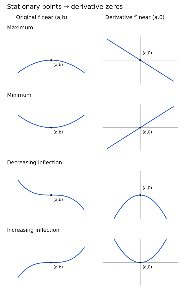
Use signs that hold on intervals on either side of the stationary input, not two sampled slopes. The source's local maximum and minimum configurations have opposite signs across the point.
- Positive → zero → negativeOriginal maximum; derivative crosses down
The original rises into the point and falls away. The derivative is above the axis on the left and below it on the right, passing through .
- Negative → zero → positiveOriginal minimum; derivative crosses up
The original falls into the point and rises away. The derivative changes from negative to positive through .
These are the sign-changing local configurations shown in the source. A derivative zero by itself does not establish a turning point.
Same signs give a touch at zero
Here the derivative is zero at the stationary input and has one strict sign throughout each neighbouring interval. The original keeps its direction through the point.
Expand diagramFit diagram to page
Use the scrollbars or arrow keys to inspect details. The text explanation follows.
- Positive → zero → positiveDerivative minimum at zero
The derivative is positive nearby and zero at the point: it touches from above. The source’s rising stationary-inflection configuration has this pattern.
- Negative → zero → negativeDerivative maximum at zero
The derivative is negative nearby and zero at the point: it touches from below. The source’s falling stationary-inflection configuration has this pattern.
Same-sign first derivatives show no original turning point. Confirm a change of the original curve’s concavity before calling it an inflection; the sign pattern alone is insufficient. The worked cubics below establish that extra condition.
Try a worked example
Read a case, make a prediction, then reveal the reasoning. The examples keep their stated values.
A maximum above the axis
Consider this illustrative function:
At input zero, predict the derivative’s height and crossing direction. Does the original height 2 carry across?
Show reasoning
1. Transfer the slope, keeping the input
The original point is (0, 2). Its slope is zero, so the derivative point is (0, 0).
2. Read both intervals
For every , ; for every , . The derivative crosses down through zero. The original curve has a strict local maximum at .
A minimum below the axis
Consider this illustrative function:
At input zero, predict where the derivative meets the axis. Does an original point below the axis force a negative derivative?
Show reasoning
1. Differentiate independently of the height
The original point is (0, -2), while its horizontal tangent gives derivative point (0, 0).
2. Read the upward crossing
For every , ; for every , . The derivative crosses from below to above. The original curve has a strict local minimum at . At , the original height is but the derivative height is : the original is below the axis while its derivative is above.
Rising on both sides
Consider this illustrative function:
At input zero, predict whether the derivative crosses or touches the axis. Then check whether the original has an inflection.
Show reasoning
1. Locate the derivative's minimum
The squared term is positive at every nonzero input, while the derivative is zero at input zero. The derivative touches zero from above and has a strict minimum there. The original point is , not .
2. Check the original concavity separately
The second derivative is negative to the left of zero and positive to the right. This change of concavity establishes the original stationary inflection. Positive first derivatives on both sides alone would not prove that change.
Falling on both sides
Consider this illustrative function:
Near input zero, predict which side of the axis contains the derivative. Is its zero a maximum or a minimum of the derivative?
Show reasoning
1. Locate the derivative's maximum
The negative squared term is negative at every nonzero input, while the derivative is zero at input zero. The derivative touches zero from below and has a strict maximum there. The original point is .
2. Confirm the original inflection
The second derivative is positive to the left of zero and negative to the right. Concavity changes, so the original point is a stationary inflection. The curve keeps falling through it; it is not an original turning point.
Compare with the paired source sketches
Expand diagramFit diagram to page
Use the scrollbars or arrow keys to inspect details.
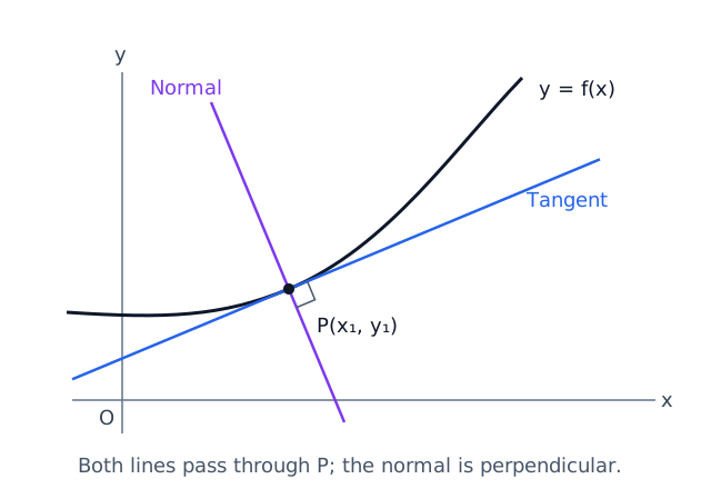
Tangent and normal through the same point
Expand diagramFit diagram to page
Use the scrollbars or arrow keys to inspect details.
Explore
Plot , and their derivatives. Before inspecting the plots, predict the stationary inputs, the increasing/decreasing intervals and which coordinates move under the translation. Compare your predictions with exact derivatives. Explain why identical derivative graphs do not determine a unique function graph without a height condition.
Related interactive example
Explore this related example, then return to the prediction task above.
Worked example
A rectangular pen stands against a straight wall, so 24 m of fencing is used for its other three sides. Let be each side perpendicular to the wall and the remaining side.
The constraint is and the area is , with . Thus , giving and .
The derivative is positive before 6 and negative after 6 on the feasible domain.
Together with area tending to zero at both ends, this establishes the greatest area of .
A stationary value is a candidate. Check the physical domain and allowed endpoints or limiting boundary behaviour before claiming an overall optimum.
Check your understanding
An open box is made from a 24 cm square sheet by cutting a square of side cm from each corner and folding up the four sides. Construct a model and find the greatest possible volume. State the feasible domain and justify that your dimensions give the greatest volume, rather than merely a stationary value.
The height is and each base side is , so for . Differentiation gives . The interior stationary input is ; would produce a degenerate box and is outside the domain.
The derivative is positive on and negative on , while volume tends to zero at both domain ends. Thus the greatest volume is , with base 16 cm by 16 cm and height 4 cm.
Mastery learning objectives
At the end of this chapter, I should be able to:
Choose a practice question
The five rows follow the printed page 53 question-type map, with links to the worked lecture examples, Discussion questions and Review problems. Use the lecture and tutorial checkpoints above to track progress.
| Common question type | Lecture examples | Discussion questions | Review follow-up |
|---|---|---|---|
| Graph of a function and its derivative | 3, 5, 6, 7 | 1, 2, 3, 4, 6(iii) | 1, 2, 3, 4, 5(iii), 6 |
| Strict increase/decrease, concavity and stationary points (maximum/minimum/inflection) | 1, 2, 4 | 5, 6(i), 6(ii) | 5(i), 5(ii) |
| Tangents and normals | 8, 9, 10, 11 | 7, 8, 9 | 7 |
| Connected rate of change | 12, 13 | 10, 13(a) | 8, 9(iv) |
| Maximisation and minimisation | 14, 15, 16 | 11, 12, 13(b) | 9(i), 9(ii), 9(iii), 10, 11, 12 |
Source qualifications: Discussion 4 asks to recover from ; its placement in the printed graph row is retained. The Discussion key on page 60 supplies selected answers only; the Review key on page 66 also omits some asks, so the linked reviewed solutions retain the complete working.
Review 5’s printed strict-decrease ranges exclude the isolated zero derivative at , while its function still strictly decreases through that point.
Review 9’s page 66 key prints square units/s, but and give : a decrease of 12. The original key is retained in the native text.
Review 12’s right-endpoint test and missing minimum area 24 are qualified and completed in its linked reviewed solution. Printed source evidence and independent corrections remain distinct.
Practice questions
Practice section 1 · Questions 1–6
Classify the turning points of a rational curve · Classify stationary points on two implicit branches · +4 more
Practice section 2 · Questions 7–12
Sketch derivative branches around two vertical asymptotes · Transfer an oblique asymptote to the derivative sketch · +4 more
Practice section 3 · Questions 13–18
Find the area between an exponential tangent and normal · Find an exact triangle area from an implicit normal · +4 more
- Find the area between an exponential tangent and normal
- Find an exact triangle area from an implicit normal
- Connect a spherical balloon’s volume and radius rates
- Find the falling water level in an inverted cone
- Minimise metal for a cylinder with a hemispherical cap
- Maximise an isosceles triangle inscribed in a circle
Practice section 4 · Questions 19–24
Minimise the metal in a fixed-volume cylindrical can · Match a function to its derivative · +4 more
Practice section 5 · Questions 25–30
Recover a function from its gradient and one value · Find horizontal and vertical tangents to a closed curve · +4 more
- Recover a function from its gradient and one value
- Find horizontal and vertical tangents to a closed curve
- Find a logarithmic tangent and a two-intersection slope range
- Use implicit tangents and a normal to bound an area
- Differentiate a triangle constrained to fixed area
- Optimise a rectangle inside a semicircle
Practice section 6 · Questions 31–36
Minimise the cone circumscribed about a sphere · Combine a leaking cone with trapezium optimisation · +4 more
- Minimise the cone circumscribed about a sphere
- Combine a leaking cone with trapezium optimisation
- Sketch a derivative across two vertical asymptotes
- Sketch the gradient across a pole and a minimum
- Differentiate turning points and a stationary inflection
- Read a derivative from an oblique asymptote and two extrema
Practice section 7 · Questions 37–42
Reconstruct a decreasing function with an isolated zero gradient · Determine a rational curve and sketch its derivative exactly · +4 more
- Reconstruct a decreasing function with an isolated zero gradient
- Determine a rational curve and sketch its derivative exactly
- Identify the parabola touched by every line in a family
- Convert units before differentiating a conical pile
- Optimise and differentiate a triangle on an implicit curve
- Optimise a flower-bed under a wall-building time budget
Practice section 8 · Questions 43–44
Maximise a complete globe on a closed cylindrical base · Optimise corner flower crates around a central pond
More practice
Draw the situation and define the quantities before choosing a derivative. Check units, the feasible domain and the justification for the requested maximum, minimum or rate.
Ready to try this on your own?
For “Applications of differentiation”, try a question without the working and explain your method. This records your confidence, saved in this browser only.